SINGLE OBJECT DETECTION PART - 1

ML MODEL TO DETECT THE BIGGEST OBJECT IN AN IMAGE — PART 1

1 - Drawing the bounding box around the largest object in an Image. It is about getting the Image Data ready for analysis.

(Read Part 2 here)

Welcome to the Part 2 of fast.ai. where we will deal with Single Object Detection . Before we start , I would like to thank Jeremy Howard and Rachel Thomas for their efforts to democratize AI.

This part assumes you to have good understanding of the Part 1. Here are the links , feel free to explore the first Part of this Series in the following order.

1. Dog Vs Cat Image Classification
2. Dog Breed Image Classification
3. Multi-label Image Classification
4. Time Series Analysis using Neural Network
5. NLP- Sentiment Analysis on IMDB Movie Dataset
6. Basic of Movie Recommendation System
7. Collaborative Filtering from Scratch
8. Collaborative Filtering using Neural Network
9. Writing Philosophy like Nietzsche
10. Performance of Different Neural Network on Cifar-10 dataset

This blog post has been divided into two parts.

• The first part starts with familiarizing yourself with the format in which data is present for Object Detection to localization of Object.
• The second part deals with Largest Item Classifier in an Image .

The dataset we will be using is PASCAL VOC (2007 version).

Lets get our hands dirty with the coding part.

As in the case of all Machine Learning projects , there are three things to focus on :-

1. Provide Data.
2. Pick some suitable Architecture .
3. Choose a Loss function.

Step 1 will focus on getting the data in proper shape so as to do analysis on top of it.

STEP 1:- It involves classifying and localizing the largest object in each image. The step involves:-

• Classifying the object.
• Locating the object.
• Labeling the located object.
• Then we will try to do all the above three steps in one go .

1.1. INSTALL THE PACKAGES

Lets install the packages and download the data using the commands as shown below.

# Install the packages# !pip install https://github.com/fastai/fastai/archive/master.zip!pip install fastai==0.7.0!pip install torchtext==0.2.3!pip install opencv-python!apt update && apt install -y libsm6 libxext6!pip3 install http://download.pytorch.org/whl/cu80/torch-0.3.0.post4-cp36-cp36m-linux_x86_64.whl !pip3 install torchvision

# Download the Data to the required folder!mkdir data!wget http://pjreddie.com/media/files/VOCtrainval_06-Nov-2007.tar -P data/!wget https://storage.googleapis.com/coco-dataset/external/PASCAL_VOC.zip -P data/!tar -xf data/VOCtrainval_06-Nov-2007.tar -C data/!unzip data/PASCAL_VOC.zip -d data/!rm -rf data/PASCAL_VOC.zip data/VOCtrainval_06-Nov-2007.tar

%matplotlib inline%reload_ext autoreload%autoreload 2

!pip install Pillow

from fastai.conv_learner import *from fastai.dataset import *

from pathlib import Pathimport jsonimport PILfrom matplotlib import patches, patheffects

Lets check what’s present in our data. We will be using the python 3 standard library pathlib for our paths and file access .

1.2. KNOW YOUR DATA USING Pathlib OBJECT.

The data folder contains different versions of Pascal VOC .

PATH = Path('data')list((PATH/'PASCAL_VOC').iterdir())# iterdir() helps in iterating through the directory of PASCAL_VOC

• The PATH is an object oriented access to directory or file. Its a part of python library pathlib. To know how to leverage the use of pathlib function do a PATH.TAB .
• Since we will be working only with pascal_train2007.json , Let’s check out the content of this file.

training_json = json.load((PATH/'PASCAL_VOC''pascal_train2007.json').open())# training_json is a dictionary variable.# As we can see Pathlib object has an open method .# json.load is a part of Json (Java Script Object Notation) library that # we have imported earlier.

training_json.keys()

This file contains the Images , Type , Annotations and Categories. For making use of Tab Completion , save it in appropriate variable name.

IMAGES,ANNOTATIONS,CATEGORIES = ['images', 'annotations', 'categories']

Lets see in detail what each of these has in detail:-

• The IMAGES consist of image name , its height , width and image id.

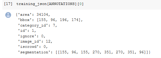
• The ANNOTATIONS consist of area, bbox(bounding box), category_id (Each category id has a class or a name associated with it ).
• Some of the images has polygon segmentation i.e the Bounding box around the object in the image. Its not important to our discussion.
• The ignore flag says to ignore the object in the image if the ignore flag=1 (True).

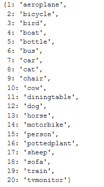
• The CATEGORIES consists of class(name) and an ID associated with it.

For easy access to all of these , lets convert the important stuffs into dictionary comprehension and list comprehension.

FILE_NAME,ID,IMG_ID,CATEGORY_ID,BBOX = 'file_name','id','image_id','category_id','bbox'

categories = {o[ID]:o['name'] for o in training_json[CATEGORIES]}# The categories is a dictionary having  class and an ID associated with # it.# Lets check out all of the 20 categories using the command belowcategories

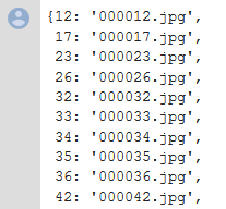
training_filenames = {o[ID]:o[FILE_NAME] for o in training_json[IMAGES]}training_filenames # contains the id and the filename of the images.

training_ids = [o[ID] for o in training_json[IMAGES]]training_ids # This is a list comprehension.

Now , lets check out the folder where we have all the images .

list((PATH/'VOCdevkit'/'VOC2007').iterdir())# The JPEGImages in red is the one with all the Images in it.

JPEGS = 'VOCdevkit/VOC2007/JPEGImages'IMG_PATH = PATH/JPEGS# Set the path of the Images as IMG_PATHlist(IMG_PATH.iterdir())[:5]# Check out all the Images in the Path

Note:- Each image has an unique id associated with it as shown above.

1.3. BOUNDING BOX

The main objective here is to bring our bounding box to proper format such that which can be used for plotting purpose. The bounding box coordinates are present in the annotations.

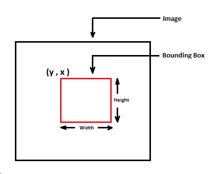
A bounding box is a box around the objects in an Image.

Earlier the Bounding box coordinates represents (column, rows, height, width). Check out the image below.

• After passing the coordinates via hw_bb() function which is used to convert height_width to bounding_box, we get the coordinates of the top left and bottom right corner and in the form of (rows and columns).

def hw_bb(bb): return np.array([bb[1], bb[0], bb[3]+bb[1]-1, bb[2]+bb[0]-1])

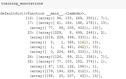
• Now , we will create a dictionary which has the image id as the key and its bounding box coordinate and the category_id as the values.

# Python's defaultdict is useful any time you want to have a default     # dictionary entry for new keys. If you try and access a key that doesn’t # exist, it magically makes itself exist and # it sets itself equal to the return value of the function you specify   # (in this case lambda:[]).training_annotations = collections.defaultdict(lambda:[])for o in training_json[ANNOTATIONS]:    if not o['ignore']:        bb = o[BBOX]        bb = hw_bb(bb)        training_annotations[o[IMG_ID]].append((bb,o[CATEGORY_ID]))

• In the above chunk of code, we are going through all the annotations , and considering those which doesn’t say ignore . After that we append it to a dictionary where the values are the Bounding box (bbox )and the category_id(class) to its corresponding image id which is the key.
• One problem is that if there is no dictionary item that exist yet, then we can’t append any list of bbox and class to it . To resolve this issue we are making use of Python’s defaultdict using the below line of code.

training_annotations = collections.defaultdict(lambda:[])

• Its a dictionary but if we are accessing a key that isn’t present , then defaultdict magically creates one and sets itself equals to the value that the function returns . In this case its an empty list. So every time we access the keys in the training annotations and if it doesn’t exist , defaultdict makes a new empty list and we can append to it.

SUMMARY OF THE USEFUL IMAGE RELATED INFORMATION

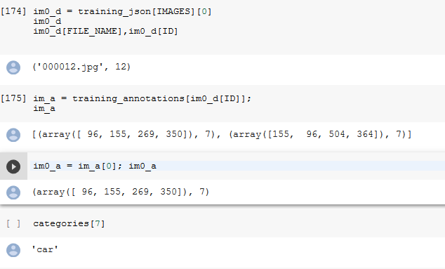
Lets get into the details of the annotations of a particular image. As we can see in the snapshot below .

• We take a particular image.
• Get its annotation i.e the Bounding Box and the Class of the Object in the BBox. It means what are the objects present in the class along with the coordinates of the objects.
• Check what does that class refers to in the below example. In this case the class or the category is a car.

Some libraries take VOC format bounding boxes, so the bb_hw() function helps in resetting the dimension into original format:

bb_voc = [155, 96, 196, 174]bb_fastai = hw_bb(bb_voc) 

# We won't be using the below function for now .def bb_hw(a): return np.array([a[1],a[0],a[3]-a[1]+1,a[2]-a[0]+1])

1.4. PLOTTING OF THE BOUNDING BOX AROUND THE OBJECT

Now we will focus on creating a bounding box around an image . For that we will create plots in steps or in separate functions . Each step serves a definite purpose towards creating a plot. Lets see the purpose of each and every step . Post that we will focus on the flow .

• The below code is used to get the axis on top of which we will plot a image .

def show_img(im, figsize=None, ax=None):# The ax is used to pass in an axis object.    if not ax: fig,ax = plt.subplots(figsize=figsize)   ax.imshow(im)   ax.get_xaxis().set_visible(False)   ax.get_yaxis().set_visible(False)   return ax

• Draw a rectangle around the object in the image using the following code.

def draw_rect(ax, b):    patch = ax.add_patch(patches.Rectangle(b[:2], *b[-2:], fill=False, edgecolor='white', lw=2))    draw_outline(patch, 4)

# *b[-2:] in the argument list is the splat operator . It passes b[-2],b[-1] as parameters. Its a shortcut.

• The draw_outline() is used to make the text visible regardless of the background. So here we are using white text with black outline or vice-versa.

def draw_outline(o, lw):    o.set_path_effects([patheffects.Stroke(        linewidth=lw, foreground='black'), patheffects.Normal()])

# foreground='black' means to create a black stroke around it.

• Write the class or category to which the image belongs, in form of text near the bounding box.

def draw_text(ax, xy, txt, sz=14):    text = ax.text(*xy, txt,        verticalalignment='top', color='white', fontsize=sz, weight='bold')    draw_outline(text, 1)

# Add text and draw outline around it.

• Here is the flow on how to create a bounding box around the object in an image.

# Step 1 :- Returns the axis the image is on by calling the function     # show_img().ax = show_img(im)# Step 2 :- Convert the bounding box coordinates into proper format by   # calling the function bb_hw().b = bb_hw(im0_a[0])# Step 3:- Draw a rectangle /Bounding box around the object by calling   # the function draw_rect().draw_rect(ax, b)# Step 4:- Draw the text near the top left corner b[:2] .# And it contains two things , the bounding box  and the class ,# im0_a[1] is the class and to get the text , pass it into               # categories[im0_a[1]]# by calling the function draw_text().draw_text(ax, b[:2], categories[im0_a[1]]) 

Let’s wrap up the flow steps, in functions as shown below:-

def draw_im(im, ann):    ax = show_img(im, figsize=(16,8))    for b,c in ann: # Destructure the annotations into bbox and class        b = bb_hw(b) # Convert it into appropriate coordinates        draw_rect(ax, b) # Draw rectangle bbox around it.        draw_text(ax, b[:2], categories[c], sz=16)         # Write some text around it

def draw_idx(i):    im_a = training_annotations[i] # Grab the annotations with the help of the image id.    im = open_image(IMG_PATH/training_filenames[i]) # Open that Image    print(im.shape) # Print its shape    draw_im(im, im_a) # Call the draw and print its text

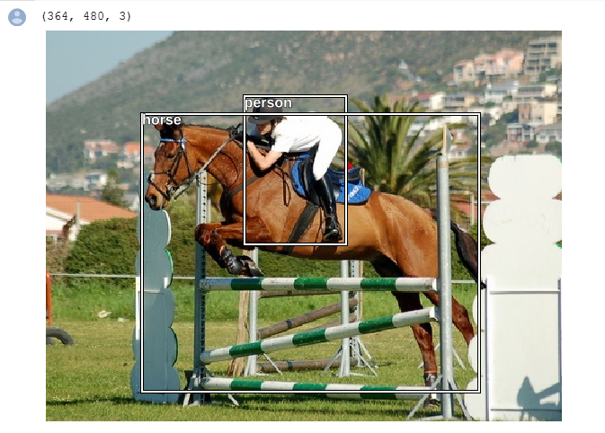
draw_idx(17) # Draw an image of a particular index.

Let’s wrap up of the flow in detail here:-

• draw_idx(17) calls the def draw_idx(i): function which grabs the annotations of image no 17 that has been passed to this function.
• Note :- Annotations of an object is the bounding box of the object in that image and the class to which the object belongs to.
• Within the def draw_idx(i) function , after grabbing the annotations , we are opening that image , printing out its shape.
• Then we call the def draw_im(im, im_a) function with the image and its annotations.
• Within this def draw_im(im, im_a) function , first we print the image .
• Then within the for loop we go through each of the annotations , store the bounding box and class in b and c respectively. This is also known as destructuring of the assignment.
• Turns the bounding box coordinates into appropriate coordinates i.e top left and bottom right corner coordinates using this bb_hw(b) function.
• draw_rect(ax, b) :- Using this function we draw a rectangle around the bounding box .
• draw_text(ax, b[:2], categories[c], sz=16):- Using this function, we are write some text .

This is how we are locating the objects in the Images. The next step is to Classify the Largest Item in the Image. We will discuss the next step in detail in the next blog Post .

A Big Shout-out to Anwesh Satapathy and Sharwon Pius for illustrating this problem in a simple way . Please check out his github Repo and the simplified roadmap to Single object Detection .

If you have any queries feel free to shoot them @ashiskumarpanda on twitter or please check it out on fastai forums.

If you see the 👏 👏 button and you like this post , feel free to do the needful 😄😄😄😄😄 .

It is a really good feeling to get appreciated by Jeremy Howard. Check out what he has to say about the Fast.ai Part 1 blog of mine . Make sure to have a look at it.

body[data-twttr-rendered="true"] {background-color: transparent;}.twitter-tweet {margin: auto !important;}

Great summary of the 2018 version of https://t.co/aQsW5afov6 - thanks for sharing @ashiskumarpanda ! https://t.co/jVUzpzp4EO

 — @jeremyphoward

SINGLE OBJECT DETECTION PART - 1 was originally published in Hacker Noon on Medium, where people are continuing the conversation by highlighting and responding to this story.