SINGLE OBJECT DETECTION PART - 2

ML MODEL TO DETECT THE BIGGEST OBJECT IN AN IMAGE PART - 2

2- Classifying and Localizing Objects in Images with the help of Bounding Box.

(Read Part 1 here)

Welcome to the Part 2 of fast.ai . This is the 8th lesson of Fastdotai where we will deal with Single Object Detection . Before we start , I would like to thank Jeremy Howard and Rachel Thomas for their efforts to democratize AI.

The 2nd part assumes to have good understanding of the first part. Here are the links , feel free to explore the first Part of this Series in the following order.

1. Dog Vs Cat Image Classification
2. Dog Breed Image Classification
3. Multi-label Image Classification
4. Time Series Analysis using Neural Network
5. NLP- Sentiment Analysis on IMDB Movie Dataset
6. Basic of Movie Recommendation System
7. Collaborative Filtering from Scratch
8. Collaborative Filtering using Neural Network
9. Writing Philosophy like Nietzsche
10. Performance of Different Neural Network on Cifar-10 dataset

This blog post focuses on Classifying the Largest Object in the Image . The data set we will be using is PASCAL VOC (2007 version). This is a continuation of last part. Check it out at

1. Single Object Detection

Hope you folks remember what we discussed earlier.

1.5. FIND THE LARGEST OBJECT IN AN IMAGE

• As we know that each image has multiple object and multiple object comes with multiple bounding box associated with it . And our aim is to find the largest object in an image, which we can get from the area of the bounding box around the objects in an image.For that we will make use of the following Largest Item Classifier function.

# get largestdef get_largest(b):    if not b: raise Exception()    b = sorted(b, key=lambda x: np.product(x[0][-2:]-x[0][:2]), reverse=True)    return b[0]

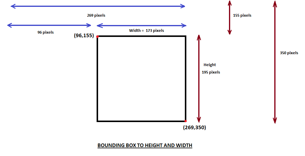
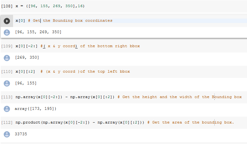
• Lets breakdown the above function . Suppose our annotations for a particular image is x = ([96, 155, 269, 350],16) .Before we proceed let me remind you , the annotation is a tuple containing the bounding box and the class to which the bounding box belongs to . The Bounding box represents the coordinates of the top left and bottom right corner. as shown below.

The below snapshot explains the above diagram in detail.

In the above function , we use the below code

b = sorted(b, key=lambda x: np.product(x[0][-2:]-x[0][:2]), reverse=True)

to get the area of all the bounding boxes present in an image and then sort it by area. b[0] returns the first bounding box i.e the largest one.

Now , lets create a dictionary where the key is Image ID and the value is a tuple containing the largest bounding box along with its class.

training_largest_annotations = {a: get_largest(b) for a,b in training_annotations.items()}training_annotations[17]

Image ID 17 contains two bounding boxes belonging to class 15 and 13. To get the largest bounding box of these two:-

training_largest_annotations[17]

1.6. PLOT THE LARGEST OBJECT IN THE IMAGE

As we have a dictionary of Image and its corresponding bbox and its class. Let’s plot this .

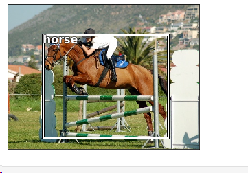
b,c = training_largest_annotations[17]b = bb_hw(b)ax = show_img(open_image(IMG_PATH/training_filenames[17]), figsize=(5,10))draw_rect(ax, b)draw_text(ax, b[:2], categories[c], sz=16)

This dictionary contains the data from which we will get our image filename and the largest class present in the image.Here we have got Horse and Person in the image .Horse being the largest object , is being plotted. Using this information we would do our modelling. Hence convert it into a .CSV file data. We use Pandas to do that.

1.7. GETTING THE DATA IN PROPER FORMAT FOR MODELLING.

• Set the Path where the CSV file should exist.

(PATH/'tmp').mkdir(exist_ok=True)CSV = PATH/'tmp/lrg.csv'

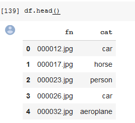
• The CSV file has two columns , one contains the Image file name (fn) and other contains the category/class to which the object in the image belongs to.

df = pd.DataFrame({'fn': [training_filenames[o] for o in training_ids],    'cat': [categories[training_largest_annotations[o][1]] for o in training_ids]}, columns=['fn','cat'])df.to_csv(CSV, index=False)

STEP 2 :- GET A SUITABLE ARCHITECTURE FOR MODELLING OF LARGEST ITEM CLASSIFIER.

In this step, we are training our model to find the largest object in a image.

f_model = resnet34sz=224bs=64

From here it’s just like Dogs vs Cats Classifier.

tfms = tfms_from_model(f_model, sz, aug_tfms=transforms_side_on, crop_type=CropType.NO)md = ImageClassifierData.from_csv(PATH, JPEGS, CSV, tfms=tfms, bs=bs)

• In tfms_from_model(...) function, we aren’t cropping hence crop_type=CropType.NO . Instead of cropping we are squishing the image.
• How do we normally resize ?? Set the smallest side to 224 and then take a random square crop during training . During validation take a center crop unless we use data augmentation . For bounding boxes , its not the same as unlike in Imagenet where the thing we care about is mostly in center and pretty big , a lot of stuff in Object detection is quite small and may be closer to the edge also.
• Using ImageClassifierData.from_csv() we are creating the model Data i.e Formatting the Data so that it can be used as per fastai format.

The squishing of the Image can be visualized using the below code snippet :-

show_img(md.val_ds.denorm(to_np(x))[0]);

Lets check our Data Loader for now:-

x,y=next(iter(md.val_dl))

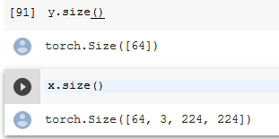
So the data loader grabs a batch of 64 images where x contains the 64 images and y contains the class this 64 images belongs to.

If we have a look into the values of x , we find that the values aren’t between 0 and 1 . Its because there is whole bunch of stuffs that is done to the input to get it ready to be passed to a pretrained model. It does some normalisation using hardcoded image statistics. To know more about these check out the transformation function using ?? tfms_from_model .

Now when we want to visualize an image from a validation data loader we have to denormalize the image as it has been normalized within the tfms_from_model . That is why we use :-

show_img(md.val_ds.denorm(to_np(x))[0]);

Denorm not only denormalizes the image but also fixes up the dimension order . Denorm is kind of undo every transformation that has been applied to md.val_ds . Pass that mini batch but you have to turn it into a numpy first .

Lets set up the Neural Network . Here f_model=resnet34 , earlier described. And optimizer used is Adam.

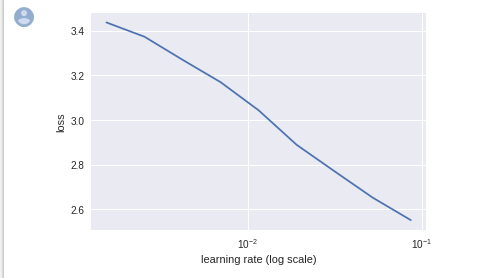
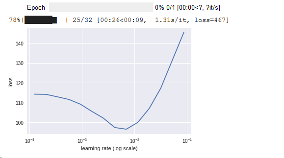
learn = ConvLearner.pretrained(f_model, md, metrics=[accuracy])learn.opt_fn = optim.Adamlrf=learn.lr_find(1e-5,100)learn.sched.plot()

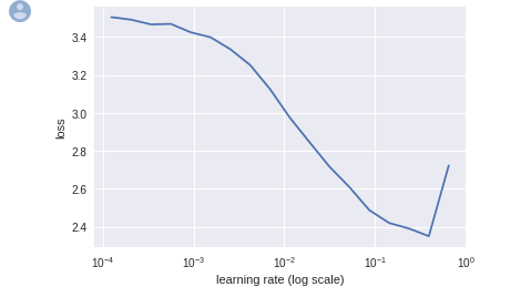
The reason we don’t see the uptick is because we have removed the first few and last few points by default. This is due to the reason the last few points actually shoots up to infinity i.e their loss is too high, so we basically cannot see anything . Hence remove it. To undo this and visualize the uptick, use the below code :-

learn.sched.plot(n_skip=5, n_skip_end=1)

What the above code does is, it skips 5 points at the start and 1 point from the end, so that all except those points can be visualized.

Lets do some training on top of this model with lr=2e-2 as visualized from this graph.

lr = 2e-2learn.fit(lr, 1, cycle_len=1)

Just training the last layer and we get an accuracy of 80%.

UNFREEZING A COUPLE OF LAYERS AND TRAINING

lrs = np.array([lr/1000,lr/100,lr])learn.freeze_to(-2)lrf=learn.lr_find(lrs/1000)learn.sched.plot(1)

learn.fit(lrs/5, 1, cycle_len=1)

Now we have reached to a better accuracy of 81%.

Unfreeze all of the layers and train:-

learn.unfreeze()learn.fit(lrs/5, 1, cycle_len=2)

Reason Why the accuracy isn’t increasing beyond 83%?

Unlike Dogs vs Cats or ImageNet where each image has one major thing. And that one major thing is what we are asked to look for. But in Pascal Datasets we have lots of little things . And so even the best classifier is not necessarily going to do great. Lets visualize the results.

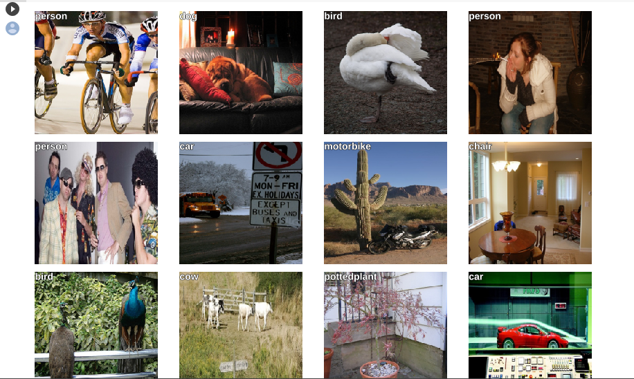
fig, axes = plt.subplots(3, 4, figsize=(12, 8))for i,ax in enumerate(axes.flat):    ima=md.val_ds.denorm(x)[i]    b = md.classes[preds[i]]    ax = show_img(ima, ax=ax)    draw_text(ax, (0,0), b)plt.tight_layout()

In the above case, our model can find the largest object in the image . Now lets put a bounding box around the largest object in the image.

STEP 3:- GET A SUITABLE ARCHITECTURE FOR MODELLING OF BOUNDING BOX AROUND THE LARGEST OBJECT IN THE IMAGE.

• How to Create a Bounding box?

For this , just need to figure out two things:-

1. Create a Neural Network with four activations that predicts four numbers i.e the bounding box edges (top left co-ordinates and bottom right co-ordinates) for the largest Object. This is a regression problem with four outputs.
2. Decide the Loss function in such a way that when it is minimized , our four predicted numbers are pretty good. Let’s see how to do this.

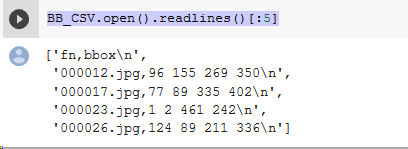
BB_CSV = PATH/'tmp/bb.csv'bb = np.array([training_largest_annotations[o][0] for o in training_ids])# Pick largest item in the image.bbs = [' '.join(str(p) for p in o) for o in bb]# Create bounding boxes separated by space.df = pd.DataFrame({'fn': [training_filenames[o] for o in training_ids], 'bbox': bbs}, columns=['fn','bbox'])# Put the image filename in one column 'fn' and bounding box of the largest object in that image in the 'bbox' columndf.to_csv(BB_CSV, index=False)# Write it in a .csv fileBB_CSV.open().readlines()[:5]# Check out how the data is stored in the below snapshot.# To do multiple label classification , the multiple labels should be space separated and file name should be comma separated.

Note:- When we are doing scaling or data augmentation to the images , that needs to be happening to the bounding box co-ordinates also.

But Why?

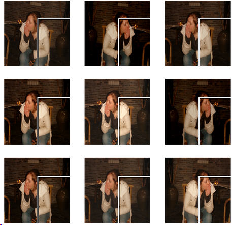
Earlier in classification case , we use to augment the images in the dataset. But there is a small change in the bounding box case. Here we have got the images and the bounding box coordinates of the objects in the images . In this case we have to augment the dependent variable i.e the bounding box coordinates as well as the image. So lets see what happens if we augment the images only .

augs = [RandomFlip(),         RandomRotate(30),        RandomLighting(0.1,0.1)]tfms = tfms_from_model(f_model, sz, crop_type=CropType.NO, aug_tfms=augs)md = ImageClassifierData.from_csv(PATH, JPEGS, BB_CSV, tfms=tfms, continuous=True, bs=4)idx=3fig,axes = plt.subplots(3,3, figsize=(9,9))for i,ax in enumerate(axes.flat):    x,y=next(iter(md.aug_dl))    ima=md.val_ds.denorm(to_np(x))[idx]    b = bb_hw(to_np(y[idx]))    print(b)    show_img(ima, ax=ax)    draw_rect(ax, b)

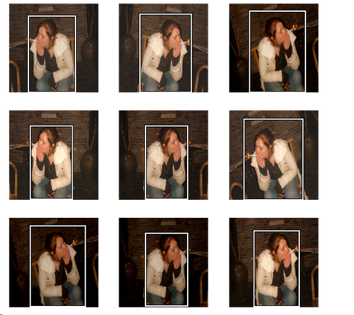
As we can see , when we are augmenting the images and not the bounding box coordinates , the images gets augmented while the bounding box representing the coordinates of the object in the image remains the same, which is not correct . This is making the data wrong. In other words, while the augmented images are changing , the bounding box representing the object in the images remains the same. Hence we need to augment the dependent variable i.e the bounding box coordinates as these two are connected to each other. The bounding box coordinates should go through all of the geometric transformation as that of the image. As can be seen in bold in the code below , we are using tfm_y=TfmType.COORD parameter which explicitly means that whatever augmentation is being done to the image should be done to the bounding box coordinates also.

augs = [RandomFlip(tfm_y=TfmType.COORD),        RandomRotate(3,p=0.5, tfm_y=TfmType.COORD),        RandomLighting(0.1,0.1, tfm_y=TfmType.COORD)]# RandomRotate parameters:- Maximum of 3 degree of rotations .p=0.5 means rotate the image half of the time.

tfms = tfms_from_model(f_model, sz, crop_type=CropType.NO, tfm_y=TfmType.COORD, aug_tfms=augs)

# Adding (tfm_y=TfmType.COORD) helps in changing the bounding box coordinates in case the model is squeezing or zooming the image

md = ImageClassifierData.from_csv(PATH, JPEGS, BB_CSV, tfms=tfms, continuous=True, bs=4)

# Note that we have to tell the transforms constructor that our labels are coordinates, so that it can handle the transforms correctly.idx=4fig,axes = plt.subplots(3,3, figsize=(9,9))for i,ax in enumerate(axes.flat):    x,y=next(iter(md.aug_dl))    ima=md.val_ds.denorm(to_np(x))[idx]    b = bb_hw(to_np(y[idx]))    print(b)    show_img(ima, ax=ax)    draw_rect(ax, b)

TfmType.COORD basically represents that if we apply flip transformation to the image , we need to change the bounding box coordinates accordingly. Hence we are adding TfmType.COORD to all the transformations that is being applied to the images.

If we see the image below ,it makes sense . The bounding box keeps on changing with the image and represents the object in the right spot.

Now, create a ConvNet based on resnet34 but here we have a twist. We don’t want any standard set of FC layers at the end that has created a classifier but instead we want to add a single layer with four output, as it’s a regression problem.

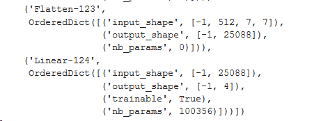
head_reg4 = nn.Sequential(Flatten(), nn.Linear(25088,4))# Append head_reg4 on top of resnet34 model which will result in creation of regressor that predicts four values as output as shown in the code below.# Here it is creating a tiny model that flattens the previous layer of the dimensions 7*7*512 =25088 and brings it down to 4 activations

learn = ConvLearner.pretrained(f_model, md, custom_head=head_reg4)learn.opt_fn = optim.Adam# Use Adam optimizer to optimize the loss function.

learn.crit = nn.L1Loss()# The loss function here is L1 loss.

The custom_head parameter in ConvLearner.pretrained(...) is added at the top of the model . It prevents creating any of the fully connected layer and adaptive maxpooling layer , which is done by default . Instead, it will replace those by whatever model we ask for. Here we want four activation representing the bounding box coordinates. We will stick this custom_head on top of the pretrained model and then train it for a while.

Check out the final layer :-

learn.summary()

After this step ,its all the same to find a best learning rate and using that learning rate , train your NN model. Lets see how it is done:-

learn.lr_find(1e-5,100)learn.sched.plot(5)

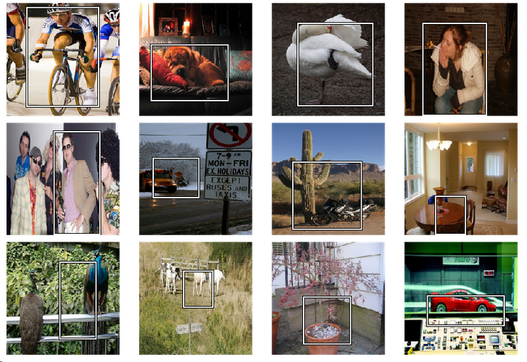
lr = 2e-3learn.fit(lr, 2, cycle_len=1, cycle_mult=2)lrs = np.array([lr/100,lr/10,lr])learn.freeze_to(-2)lrf=learn.lr_find(lrs/1000)learn.sched.plot(1)learn.fit(lrs, 2, cycle_len=1, cycle_mult=2)learn.freeze_to(-3)learn.fit(lrs, 1, cycle_len=2)learn.save('reg4')learn.load('reg4')x,y = next(iter(md.val_dl))learn.model.eval()preds = to_np(learn.model(VV(x)))

fig, axes = plt.subplots(3, 4, figsize=(12, 8))for i,ax in enumerate(axes.flat):    ima=md.val_ds.denorm(to_np(x))[i]    b = bb_hw(preds[i])    ax = show_img(ima, ax=ax)    draw_rect(ax, b)plt.tight_layout()

As seen in the above predicted output snapshot , its doing a pretty good job . Although it fails in the case of peacock and cows.

In our next blog post, we will combine Step 2 and Step 3. This will help us to predict the largest object in an image as well as the bounding box for that largest object at the same time .

There were lots of stuff covered in this blog post . You might feel like this

But that’s okay !!! I highly encourage you to go back to the previous part and check out the flow . I’ve marked the important stuffs in bold points and it will help you understand the intermediate important steps.

Thanks for sticking by this part.

In my next blog post , we will see how to combine step 2 and step 3 in a single go. Nothing new from computer vision perspective, but its the beauty of Pytorch coding which we will dive into.

Until then Good bye ..

It is a really good feeling to get appreciated by Jeremy Howard. Check out what he has to say about the Fast.ai Part 1 blog of mine . Make sure to have a look at it.

body[data-twttr-rendered="true"] {background-color: transparent;}.twitter-tweet {margin: auto !important;}

Great summary of the 2018 version of https://t.co/aQsW5afov6 - thanks for sharing @ashiskumarpanda ! https://t.co/jVUzpzp4EO

 — @jeremyphoward

SINGLE OBJECT DETECTION PART - 2 was originally published in Hacker Noon on Medium, where people are continuing the conversation by highlighting and responding to this story.