Deep Learning: Feedforward Neural Networks Explained

Feedforward neural networks are also known as Multi-layered Network of Neurons (MLN). These networks of models are called feedforward because the information only travels forward in the neural network, through the input nodes then through the hidden layers (single or many layers) and finally through the output nodes. In MLN there are no feedback connections such that the output of the network is fed back into itself. These networks are represented by a combination of many simpler models(sigmoid neurons).

Citation Note: The content and the structure of this article is based on the deep learning lectures from One-Fourth Labs — Padhai.

Motivation: Non-Linear Data

Before we talk about the feedforward neural networks, let’s understand what was the need for such neural networks. Traditional models like perceptron — which takes real inputs and give boolean output only works if the data is linearly separable. That means that the positive points (green) should lie on one side of the boundary and negative points (red) lie another side of the boundary. As you can see from the below figure perceptron is doing a very poor job of finding the best decision boundary to separate positive and negative points.

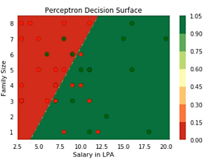Perceptron Decision Surface for Non-Linear Data

Next, we have the sigmoid neuron model this is similar to perceptron, but the sigmoid model is slightly modified such that the output from the sigmoid neuron is much smoother than the step functional output from perceptron. Although we have introduced the non-linear sigmoid neuron function, it is still not able to effectively separate red points(negatives) from green points(positives).

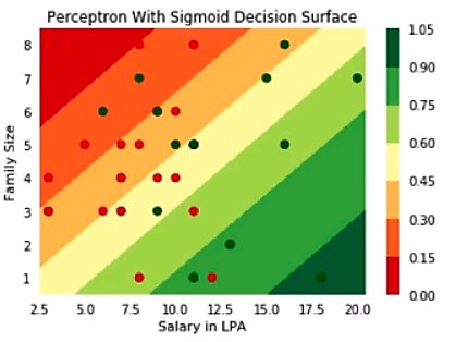Sigmoid Neuron Decision Boundary for Non-Linear Data

The important point is that from a rigid decision boundary in perceptron, we have taken our first step in the direction of creating a decision boundary that works well for non-linearly separable data. Hence the sigmoid neuron is the building block of our feedforward neural network.

From my previous post on Universal Approximation theorem, we have proved that even though single sigmoid neuron can’t deal with non-linear data. If we connect multiple sigmoid neurons in an effective way, we can approximate the combination of neurons to any complex relationship between input and the output, required to deal with non-linear data.

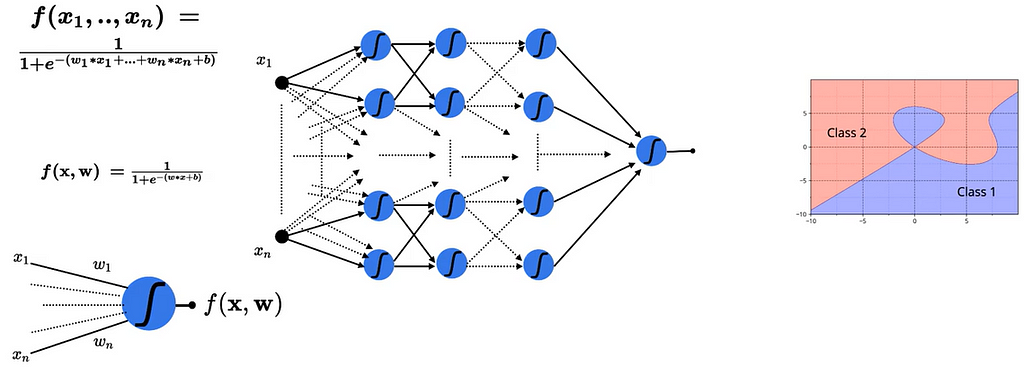Combination of Sigmoid Neurons for Non-Linear Data

Feedforward Neural Networks

Multi-layered Network of neurons is composed of many sigmoid neurons. MLNs are capable of handling the non-linearly separable data. The layers present between the input and output layers are called hidden layers. The hidden layers are used to handle the complex non-linearly separable relations between input and the output.

Simple Deep Neural Network

In this section let’s see how can we use a very simple neural network to solve complex non-linear decision boundaries.

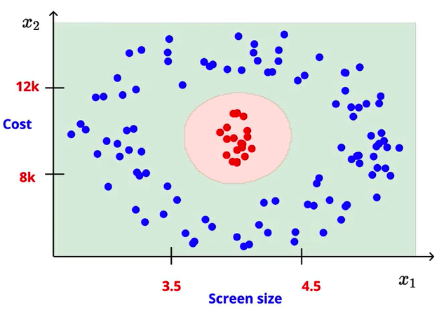
Let’s take an example of a mobile phone like/dislike predictor with two variables: screen size, and the cost. It has a complex decision boundary as shown below:

Decision Boundary

We know that by using a single sigmoid neuron, it is impossible to obtain this kind of non-linear decision boundary. Regardless of how we vary the sigmoid neuron parameters w and b. Now change the situation and use a simple network of neurons for the same problem and see how it handles.

Simple Neural Network

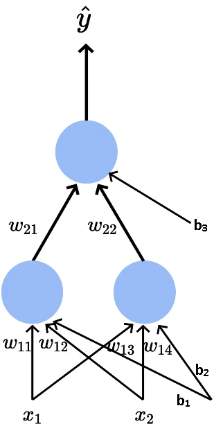
We have our inputs x₁ — screen size and x₂— price going into the network along with the bias b₁ and b₂.

Now let’s break down the model neuron by neuron to understand. We have our first neuron (leftmost) in the first layer which is connected to inputs x₁ and x₂ with the weights w₁₁ and w₁₂ and the bias b₁ and b₂. The output of that neuron represented as h₁, which is a function of x₁ and x₂ with parameters w₁₁ and w₁₂.

Output of the first Neuron

If we apply the sigmoid function to the inputs x₁ and x₂ with the appropriate weights w₁₁, w₁₂ and bias b₁ we would get an output h₁, which would be some real value between 0 and 1. The sigmoid output for the first neuron h₁ will be given by the following equation,

Output Sigmoid for First Neuron

Next up, we have another neuron in the first layer which is connected to inputs x₁ and x₂ with the weights w₁₃ and w₁₄ along with the bias b₃ and b₄. The output of the second neuron represented as h₂.

Output of the second Neuron

Similarly, the sigmoid output for the second neuron h₂ will be given by the following equation,

So far we have seen the neurons present in the first layer but we also have another output neuron which takes h₁ and h₂ as the input as opposed to the previous neurons. The output from this neuron will be the final predicted output, which is a function of h₁ and h₂. The predicted output is given by the following equation,

Complex looking Equation!! Really?. Comment if you understood it or not.

Earlier we can adjust only w₁, w₂ and b — parameters of a single sigmoid neuron. Now we can adjust the 9 parameters (w₁₁, w₁₂, w₁₃, w₁₄, w₂₁, w₂₂, b₁, b₂, b₃), which allows the handling of much complex decision boundary. By trying out the different configurations for these parameters we would be able to find the optimal surface where output for the entire middle area (red points) is one and everywhere else is zero, what we desire.

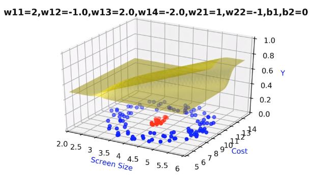Decision Boundary from Network

The important point to note is that even with the simple neural network we were able to model the complex relationship between the input and output. Now the question arises, how do we know in advance this particular configuration is good and why not add few more layers between or add few more neurons in the first layer. All these questions are valid but for now, we will keep things simple take the network as it is. We will discuss these questions and a lot more in detail when we discuss hyper-parameter tunning.

Generic Deep Neural Network

In the previous, we have seen the neural network for a specific task, now we will talk about the neural network in generic form.

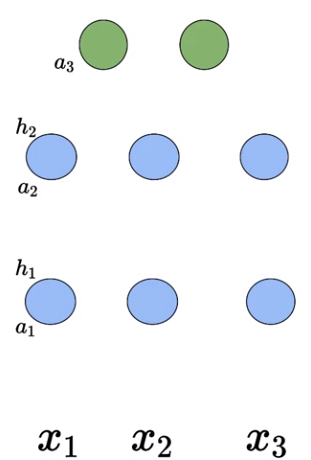Generic Network without Connections

Let’s assume we have our network of neurons with two hidden layers (in blue but there can more than 2 layers if needed) and each hidden layer has 3 sigmoid neurons there can be more neurons but for now I am keeping things simple. We have three inputs going into the network (for simplicity I used only three inputs but it can take n inputs) and there are two neurons in the output layer. As I said before we will take this network as it is and understand the intricacies of the deep neural network.

First, I will explain the terminology then we will go into how these neurons interact with each other. For each of these neurons, two things will happen

1. Pre-activation represented by ‘a’: It is a weighted sum of inputs plus the bias.
2. Activation represented by ‘h’: Activation function is Sigmoid function.

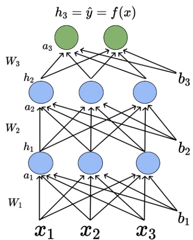Generic Network with Connections

Let’s understand the network neuron by neuron. Consider the first neuron present in the first hidden layer. The first neuron is connected to each of the inputs by weight W₁.

Going forward I will be using this format of the indices to represent the weights and biases associated with a particular neuron,

W(Layer number)(Neuron number in the layer)(Input number)

b(Layer number)(Bias number associated for that input)

W₁₁₁— Weight associated with the first neuron present in the first hidden layer connected to the first input.

W₁₁₂— Weight associated with the first neuron present in the first hidden layer connected to the second input.

b₁₁ — Bias associated with the first neuron present in the first hidden layer.

b₁₂ — Bias associated with the second neuron present in the first hidden layer.

….

Here W₁ a weight matrix containing the individual weights associated with the respective inputs. The pre-activation at each layer is the weighted sum of the inputs from the previous layer plus bias. The mathematical equation for pre-activation at each layer ‘i’ is given by,

Pre-activation Function

The activation at each layer is equal to applying the sigmoid function to the output of pre-activation of that layer. The mathematical equation for the activation at each layer ‘i’ is given by,

Activation Function

Finally, we can get the predicted output of the neural network by applying some kind of activation function (could be softmax depending on the task) to the pre-activation output of the previous layer. The equation for the predicted output is shown below,

Output Activation Function

Computations in Deep Neural Network

We have seen the terminology and functional aspect of the neural network. Now we will see how the computations inside a DNN takes place.

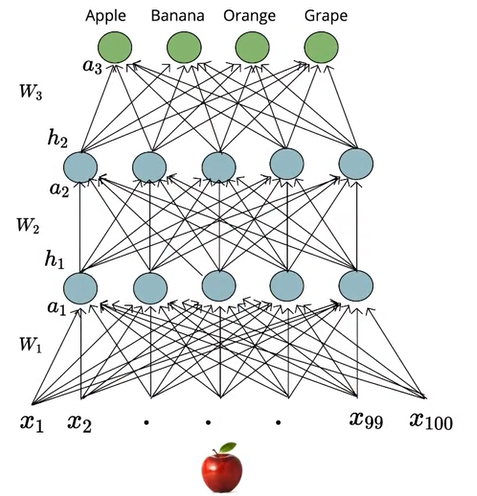
Consider that you have 100 inputs and 10 neurons in the first and second hidden layers. Each of the 100 inputs will be connected to the neurons will be The weight matrix of the first neuron W₁ will have a total of 10 x 100 weights.

Weight Matrix

Remember, we are following a very specific format for the indices of the weight and bias variable as shown below,

W(Layer number)(Neuron number in the layer)(Input number)

b(Layer number)(Bias number associated for that input)

Now let’s see how we can compute the pre-activation for the first neuron of the first layer a₁₁. We know that pre-activation is nothing but the weighted sum of inputs plus bias. In other words, it is the dot product between the first row of the weight matrix W₁ and the input matrix X plus bias b₁₁.

Similarly the pre-activation for other 9 neurons in the first layer given by,

In short, the overall pre-activation of the first layer is given by,

Where,

W₁ is a matrix containing the individual weights associated with the corresponding inputs and b₁ is a vector containing(b₁₁, b₁₂, b₁₃,….,b₁₀) the individual bias associated with the sigmoid neurons.

The activation for the first layer is given by,

Where ‘g’ represents the sigmoid function.

Remember that a₁ is a vector of 10 pre-activation values, here we are applying the element-wise sigmoid function on all these 10 values and storing them in another vector represented as h₁. Similarly, we can compute the pre-activation and activation values for ’n’ number of hidden layers present in the network.

Output Layer of DNN

So far we have talked about the computations in the hidden layer. Now we will talk about the computations in the output layer.

Generic Network with Connections

We can compute the pre-activation a₃ at the output layer by taking the dot product of weights associated W₃ and activation of the previous layer h₂ plus bias vector b₃.

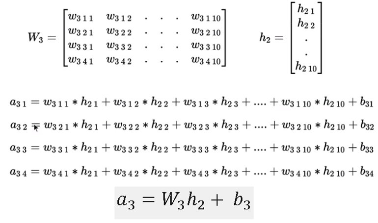Pre-activation for the output layer

To find out the predicted output from the network, we are applying some function (which we don’t know yet) to the pre-activation values.

Predicted Values

These two outputs will form a probability distribution that means their summation would be equal to 1.

The output Activation function is chosen depending on the task at hand, can be softmax or linear.

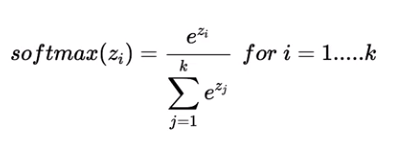
Softmax Function

We will use the Softmax function as the output activation function. The most frequently used activation function in deep learning for classification problems.

Softmax Function

In the Softmax function, the output is always positive, irrespective of the input.

Now, let us illustrate the Softmax function on the above-shown network with 4 output neurons. The output of all these 4 neurons is represented in a vector ‘a’. To this vector, we will apply our softmax activation function to get the predicted probability distribution as shown below,

Applying the Softmax Function

By applying the softmax function we would get a predicted probability distribution and our true output is also a probability distribution, we can compare these two distributions to compute the loss of the network.

Loss Function

In this section, we will talk about the loss function for binary and multi-class classification. The purpose of the loss function is to tell the model that some correction needs to be done in the learning process.

In general, the number of neurons in the output layer would be equal to the number of classes. But in the case of binary classification, we can use only one sigmoid neuron which outputs the probability P(Y=1) therefore we can obtain P(Y=0) = 1-P(Y=1). In the case of classification, We will use the cross-entropy loss to compare the predicted probability distribution and the true probability distribution.

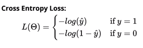
Cross-entropy loss for binary classification is given by,

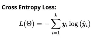
Cross-entropy loss for multi-class classification is given by,

Learning Algorithm: Non-Mathy Version

We will be looking at the non-math version of the learning algorithm using gradient descent. The objective of the learning algorithm is to determine the best possible values for the parameters, such that the overall loss of the deep neural network is minimized as much as possible.

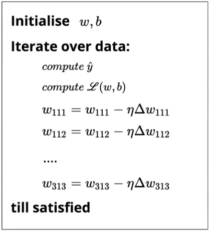
The learning algorithm goes like this,

We initialize all the weights w (w₁₁₁, w₁₁₂,…) and b (b₁, b₂,….) randomly. We then iterate over all the observations in the data, for each observation find the corresponding predicted distribution from the neural network and compute the loss using cross-entropy function. Based on the loss value, we will update the weights such that the overall loss of the model at the new parameters will be less than the current loss of the model.

Photo by Vasily Koloda on Unsplash

Conclusion

In this post, we briefly looked at the limitations of traditional models like perceptron and sigmoid neuron to handle the non-linear data and then we went on to see how we can use a simple neural network to solve complex decision boundary problem. We then looked at the neural network in a generic sense and the computations behind the neural network in detail. Finally, we have looked at the learning algorithm of the deep neural network.

Recommended Reading:

Sigmoid Neuron Learning Algorithm Explained With Math

In my next post, we will discuss how to implement the feedforward neural network from scratch in python using numpy. So make sure you follow me on medium to get notified as soon as it drops.

Until then Peace :)

NK.

Connect with me on LinkedIn or follow me on twitter for updates on future posts & discussions on the current story.

Deep Learning: Feedforward Neural Networks Explained was originally published in Hacker Noon on Medium, where people are continuing the conversation by highlighting and responding to this story.