Perceptron — Deep Learning Basics

Perceptron — Deep Learning Basics

An upgrade to McCulloch-Pitts Neuron.

Perceptron is a fundamental unit of the neural network which takes weighted inputs, process it and capable of performing binary classifications. In this post, we will discuss the working of the Perceptron Model. This is a follow-up blog post to my previous post on McCulloch-Pitts Neuron.

In 1958 Frank Rosenblatt proposed the perceptron, a more generalized computational model than the McCulloch-Pitts Neuron. The important feature in the Rosenblatt proposed perceptron was the introduction of weights for the inputs. Later in 1960s Rosenblatt’s Model was refined and perfected by Minsky and Papert. Rosenblatt’s model is called as classical perceptron and the model analyzed by Minsky and Papert is called perceptron.

Disclaimer: The content and the structure of this article is based on the deep learning lectures from One-Fourth Labs — Padhai.

Perceptron

In the MP Neuron Model, all the inputs have the same weight (same importance) while calculating the outcome and the parameter b can only take fewer values i.e., the parameter space for finding the best parameter is limited.

The proposed perceptron model introduces the concept of weights to the inputs and also devised an algorithm to find these numerical parameters. In perceptron model inputs can be real numbers unlike the boolean inputs in MP Neuron Model. The output from the model still is boolean outputs {0,1}.

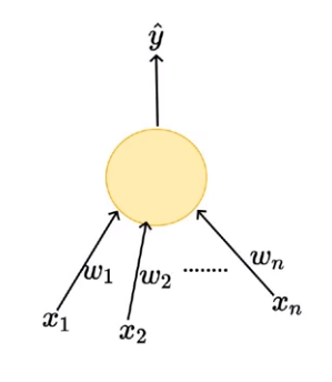Fig 1— Perceptron ModelMathematical Representation

The mathematical representation kind of looks like an if-else condition, if the weighted sum of the inputs is greater than threshold b output will be 1 else output will be 0.

Fig 2 — Mathematical Representation

The function here has two parameters weights w(w1,w2,....,wn) and threshold b. The mathematical representation of Perceptron looks an equation of a line (2D) or a plane(3D).

w1x1+w2x2-b = 0 (In 2D)w1x1+w2x2+w3x3-b = 0 (In 3D)

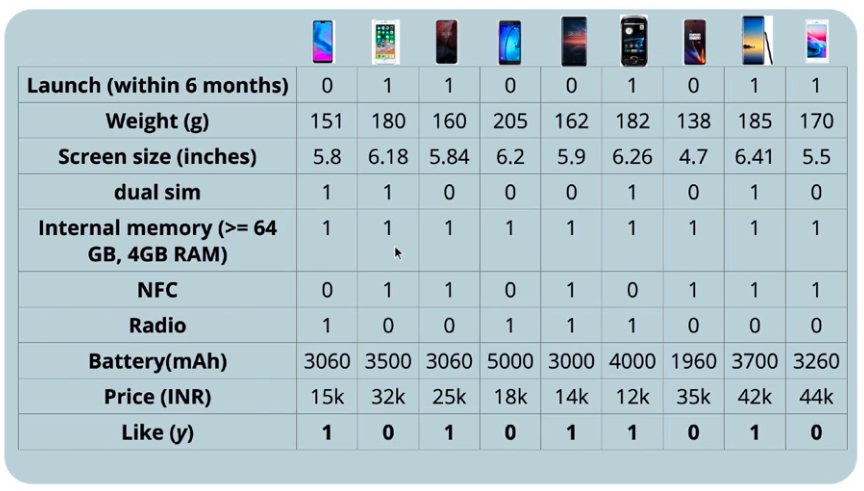
To understand the concepts of weights, let us take our previous example of buying a phone based on the information about the features of the phone. The outcome will be binary {y — 0: Not buying a phone, y — 1: buying a phone}. In this model instead of binary values for the features, we can have real numbers as the input to the model.

Fig 3 — Buying a Phone or not

Generally, the relationship between the price of a phone and likeliness to buy a phone is inversely proportional (except for a few fanboys). For someone who is an iphone fan, he/she will be more likely to buy a next version of the phone irrespective of its price. But on the other hand, an ordinary consumer may give more importance to budget offerings from other brands. The point here is, all the inputs don’t have equal importance in the decision making and weights for these features depend on the data and the task at hand.

Input Data

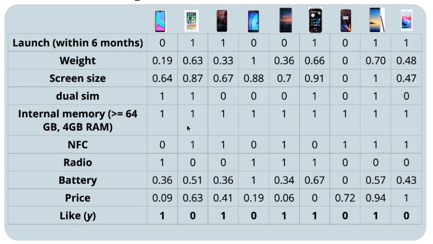
The inputs to the Perceptron model can be real numbers, because of this one obvious challenge will face is the dis-similarly of units for features i.e., not all features will be present in the same units. From the above input data, we can see that the Price is present in thousands and the Screen size is in tens. In the model, we are taking a decision by performing a weighted aggregation on all the inputs. It is very important to have all the features present in the data to be on the same scale and so that these features will have the same importance, at least in the initial stage of iteration. In order to bring all the features to the same scale. We will perform min-max standardization to bring all the values to a range 0–1.

Fig 4 — Standardized data

Loss Function

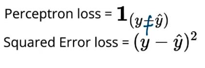
The purpose of the loss function is to tell the model that some correction needs to be done in the learning process. Let’s consider that we are making a decision based on only two features, Weight and Screen size.

Fig 5— Smaller data set

The loss function value will be zero if the Yactual and Ypredicted are equal else it will be 1. This can be represented using an indicator variable, value of the variable will be 1 if Yactual and Ypredicted are not equal else it will be 0.

Fig 6— Perceptron Loss

Learning Algorithm

Before we discuss the learning algorithm, once again let's look at the perceptron model in its mathematical form. In the case of two features, I can write the equation shown in Fig — 2 as,

w2x2+w1x1-b ≥ 0lets say, w0 = -b and x0 = 1 then,w2x2+w1x1+w0x0 ≥ 0.

Generalizing the above equation for n features as shown below,

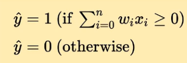Fig 7— Modified Mathematical representation

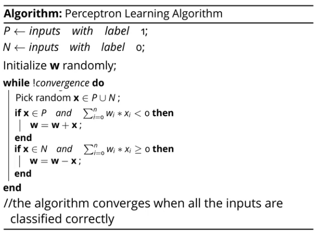
The main goal of the learning algorithm is to find vector w capable of absolutely separating both sets of data. Training data contains two sets of inputs, P (Positive y = 1) and N (Negative y = 0). Perceptron learning algorithm goes like this,

Fig 8— Perceptron Algorithm

We initialize the weights randomly, then pick a random observation x from the entire data. If the x belongs to the positive class and the dot product w.x < 0 it means that the model is making an error (we need the output to be w.x ≥ 0 for positive class refer Fig — 6) and the weights need to be updated (w = w + x). Similarly, if the x belongs to the negative class and the dot product w.x ≥ 0 (we need the output to be w.x < 0 for negative class) again in this case the model made an error, so the weights need to be updated (w = w — x). We will continue this operation till we reach convergence, convergence in our case means that our model is able to classify all the inputs correctly.

The intuition behind the Learning Algorithm

We saw how the weights are getting updated whenever there is a miss-classification. Now we will see why updating the weights (adding or subtracting) helps us to classify positive and negative classes perfectly.

To understand this concept lets go back to a bit of geometry and linear algebra. The cosine angle between the two vectors w and u is given by

w.u =∥w∥∥u∥cos(θ)Where θ is the angle between x and w, with 0≤θ≤180°cos(θ) ranges from 1 to -1, for θ = 0° and θ = 180° respectively

The important point to note from the cosine formula is that the sign of the cosine angle depends on the dot product between the two vectors because the L2 norm or the magnitude is always positive even if the vector elements are negative.

If w.x > 0, then θ < 90 => cos(θ) > 0; acute angleIf w.x < 0, then θ > 90 => cos(θ) < 0; obtuse angle

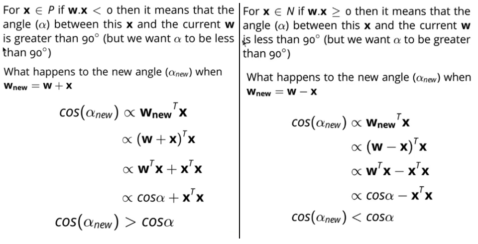
With this intuition, let's go back to the update rule and see how it works. For all observations x belongs to positive input space P, we want the w.x ≥ 0 that means the angle between the two vectors w and x should be less than 90. In case there is a miss-classification, we are updating the parameters by adding the x to w. Essentially we are increasing the cosine angle between w and x, if the cosine angle is increasing that means the angle between vectors decreases from obtuse to acute, which is what we wanted.

Fig 9— Update algorithm

Similarly, for observations belonging to negative input space N, we want dot product w.x < 0. In case there is a miss-classification, we are reducing the weights to reduce the cosine angle between the Wnew and x. If the cosine angle is decreasing that means the angle between the vectors increases from acute to obtuse, which is what we wanted.

Model Evaluation

Once we got the best weights w from the learning algorithm, we can evaluate the model on the test data by comparing the actual class of observation and the predicted class of the observation.

Fig 10 — Testing data

For evaluation, we will calculate the accuracy score of the model.

Fig 11 — Accuracy score

Conclusion

In this post, we looked at the Perceptron Model and compared it the MP Neuron Model. We also looked at the Perceptron Learning Algorithm and the intuition behind why the updating weights Algorithm works.

In the next post, we will implement the perceptron model from scratch using python and breast cancer data set present in sklearn. Stay tuned for that.

Connect with MeGitHub: https://github.com/Niranjankumar-c LinkedIn: https://www.linkedin.com/in/niranjankumar-c/

Perceptron — Deep Learning Basics was originally published in Hacker Noon on Medium, where people are continuing the conversation by highlighting and responding to this story.