Some State of the Art Optimizers in Neural Networks

We are going to study Momentum, Nesterov Accelerated Momentum, AdaGrad, AdaDelta, RMSProp, Adam, AdaMax, AMSGrad.

Optimization is the heart of Machine learning

Before begin on our topic, let’s understand..

Why do we need Optimization?

According to Merriam-Webster dictionary, meaning of the word optimize is “to make as perfect, effective, or functional as possible”. This is the definition to understand why we need Optimization in neural networks.

So in machine learning, we perform optimization on the training data and check its performance on a new validation data.

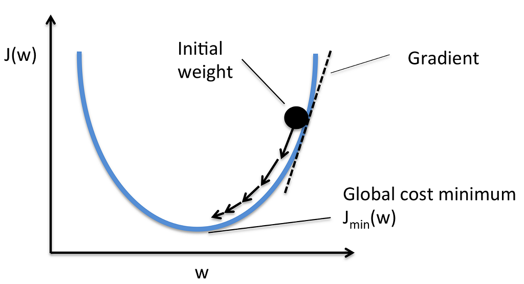
We already have a cost function which will tell us about the behavior of our model. Initially, our model contains arbitrary defined parameters like weights and biases and now we need to find the best possible state of those parameters to make a good prediction of unseen data and to do that we need some sort of a mechanism to update the parameters.

Now, we do this by a base technique called Gradient Descent. In this technique weights are updated by the following method :

J(w) is same as J(θ)

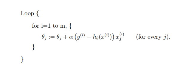
Note- In Gradient Descent, we take the whole training set into consideration in an epoch (i.e once every input data is analysed then we update the parameters) but in Stochastic Gradient Descent we take a single data input at a time (i.e once an input data is analysed then we update the parameters).

A little more about Stochastic Gradient Descent :

In this algorithm, we repeatedly run through the training set, and each time we encounter a training example, we update the parameters according to the gradient of the error with respect to that single training example only.

We now have basic understanding of Optimizers. Now, we are able to understand some State of the Art Optimizers. So, let’s begin.

Momentum

Just alone Gradient Descent does not work well in scenarios like steep gorge(local minima). Thus, making slow progress around the local minima.

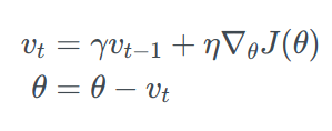
Momentum is a method that helps accelerate SGD in the right direction and dampens oscillations. It adds a fraction γ of the update vector of the past time step to the current update vector.

The momentum term increases for dimensions whose gradients point in the same directions and reduces updates for dimensions whose gradients change directions.

Nesterov Accelerated Momentum

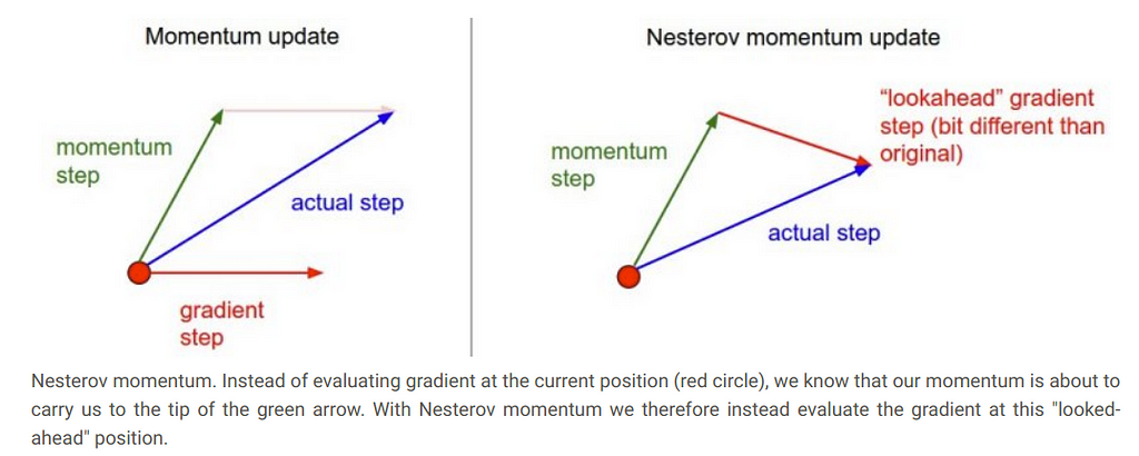
The problem with Momentum is that around the local minima its value is so high that it overshoots the minima and again continues to find local minima resulting in an ever going process.So, to make the momentum in check Nesterov suggested Nesterov Accelerated Momentum .

The core idea behind Nesterov accelerated momentum is that when the current parameter vector is at some position x, then looking at the momentum update above, we know that the momentum term alone (i.e. ignoring the second term with the gradient) is about to nudge the parameter vector by mu * v. Therefore, if we are about to compute the gradient, we can treat the future approximate position x + mu * v as a “lookahead” - this is a point in the vicinity of where we are soon going to end up. Hence, it makes sense to compute the gradient at x + mu * v instead of at the “old/stale” position x.

AdaGrad(Adaptive Gradient)

AdaGrad allows the learning rate to adapt based on the parameters.

Gt ∈ ℝd×d here is a diagonal matrix where each diagonal element i,i is the sum of the squares of the gradients w.r.t. θi up to time step t, while ϵ is a smoothing term that avoids division by zero (usually on the order of 1e−8)

The main benefit of using AdaGrad is that it eliminates the need to manually tune the learning rate. Just set the learning rate to 0.01 and leave it that way the algorithm will update it at every time step.

It’s main weakness is its accumulation of the squared gradients in the denominator: Since every added term is positive, the accumulated sum keeps growing during training. This in turn causes the learning rate to shrink and eventually become infinitesimally small, at which point the algorithm is no longer able to acquire additional knowledge.

AdaDelta

To reduce the aggressiveness, strictly decreasing learning rate of AdaGrad, AdaDelta is used. Instead of accumulating all past squared gradients, it holds the accumulated past gradients to some fixed size w.

Instead of storing w previous squared gradients, the sum of gradients is recursively defined as a decaying average of all past squared gradients.

We set γ to around 0.9

RMSProp

The only difference between RMSProp and AdaDelta is that a term mₜ⁺₁ is introduced.

RMSprop and Adadelta have both been developed independently around the same time developed for the need to resolve Adagrad’s radically diminishing learning rates. RMSProp is proposed by Geoff Hinton but it remained unpublished.

Adam(Adaptive Moment Estimation)

Adam is another algorithm that computes adaptive learning rates(η) of each parameter. The main difference is that instead of just storing an exponentially decaying average of past gradients (mₜ) like momentum it also stores exponentially decaying average of past squared gradients (vₜ) like RMSProp and AdaDelta.

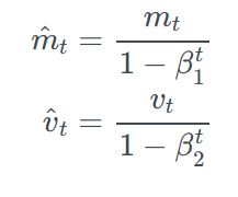
As mₜ and vₜ are initialized as 0 vectors, they are biased towards 0, and especially when the decay rates are small (i.e. β₁ and β₂ are close to 1). Therefore, to overcome this issue mₜ cap and vₜ cap is calculated.

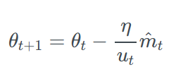
Now, we just have to write an expression for updating our parameters as we did in other optimizers.

AdaMax

Adamax is a variant of Adam based on the infinity norm. In Adam update rule scales the gradient inversely proportionally to the 𝔩₂ norm of the past gradients (vₜ-₁) and the current gradient term(|gₜ|²) instead of this we can generalize the update to the 𝔩ₚ norm.

putting p →∞ ,

To avoid confusion with Adam, uₜ is used to define the infinity norm-constraint instead of vₜ:

Finally, we can now put this uₜ in the Adam update equation by replacing with √^vₜ + ϵ :

Note that as uₜ relies on the max operation, it is not as suggestible to bias towards zero as mₜ and vₜ in Adam, which is why we do not need to compute a bias correction for uₜ. Good default values are again η=0.002, β₁=0.9 and β₂=0.999 .

AMSGrad

AMSGrad uses the maximum of past squared gradients vₜ rather than the exponential average to update the parameters.

The full AMSGrad update is :

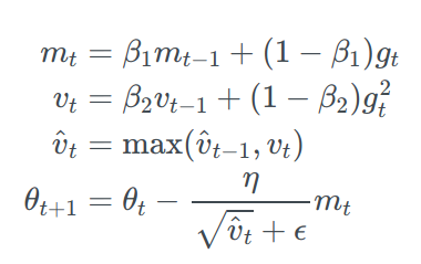For simplicity, the authors remove the debiasing step that we have seen in Adam. The only reason biasing is introduced in the first place is because we don’t want our model to become bias towards 0 so to prevent this we use biasing.

Which Optimizer to use and when ?

Not every Optimizer is good for every situation we need to determine which optimizer is best according to our task.

Some optimizer works better in Computer Vision tasks, others works better when it comes to RNNs and some of them are better when the input data is sparse.

The main benefit of adaptive learning-rate(η) based optimizers is that we don’t need to tune learning-rate but we still can achieve best results with the default values.

Summary, RMSprop is an extension of AdaGrad that deals with its rapidly diminishing learning rates. It is very identical to AdaDelta, except that AdaDelta uses the RMS of parameter updates in the numerator update rule. Adam, finally, adds bias-correction and momentum to RMSprop. RMSprop, AdaDelta, and Adam are very similar algorithms that do well in similar circumstances. The bias-correction helps Adam slightly outperform RMSprop towards the end of optimization as gradients become sparser.

So far, Adam might be the best overall choice.

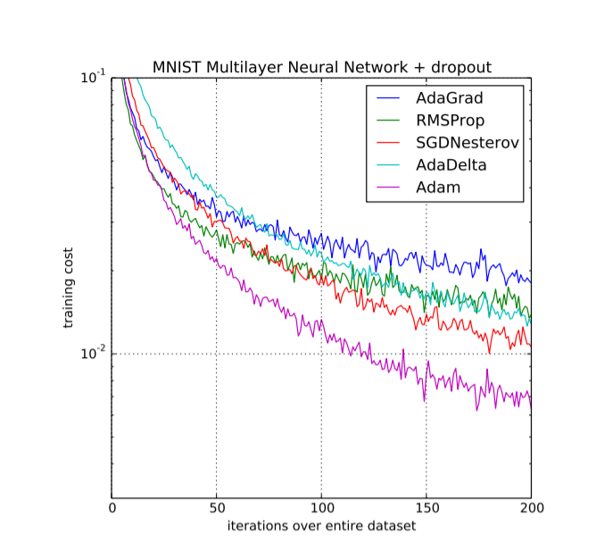Reference taken from ADAM: A METHOD FOR STOCHASTIC OPTIMIZATION

For preventing the learning rates to become infinitesimally small as training progresses, AdaDelta introduces the concept of exponential average of squared gradients upto a fixed ω. However, this short-term memory of gradients becomes an obstacle in other ways. Adam also uses this short-term memory feature.

It has been observed that some minibatches provide large and important gradients but occurs rarely resulting diminishing their influence, which leads to poor convergence. To solve this issue AMSgrad is used which uses the maximum of past squared gradients vₜ rather than the exponential average to update the parameters.

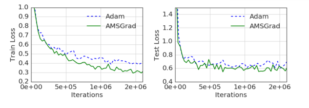the two plots compare the training and test loss of ADAM and AMSGRAD with respect to the iterations for CIFARNET. Reference is taken from ON THE CONVERGENCE OF ADAM AND BEYOND

References

[1] http://proceedings.mlr.press/v28/sutskever13.pdf

[2] http://www.jmlr.org/papers/volume12/duchi11a/duchi11a.pdf

[3] https://arxiv.org/pdf/1212.5701.pdf

[4] https://arxiv.org/pdf/1412.6980.pdf

[5]https://www.sciencedirect.com/science/article/pii/S0893608098001166?via%3Dihub

[6] https://keras.io/optimizers/

[7] http://www.satyenkale.com/papers/amsgrad.pdf

Some State of the Art Optimizers in Neural Networks was originally published in Hacker Noon on Medium, where people are continuing the conversation by highlighting and responding to this story.