Logistic Regression in Python from scratch

Logistic Regression in Python (A-Z) from Scratch

Classification is a very common and important variant among Machine Learning Problems. Many Machine Algorithms have been framed to tackle classification (discrete not continuous) problems. Examples of classification based predictive analytics problems are:

1. Diabetic Retinopathy: Given a retinal image, classify the image (eye) as Diabetic or Non-Diabetic.
2. Sentiment Analysis: Given a sentence, analyze the sense of the sentence (for ex. happiness/sadness, praise/insult, etc.)
3. Digit Recognition: Given an image of a digit, recognize the digit (0–9). This is an example of Multi-Class Classification.

and many more…

Problems 1 and 2 are examples of Binary Classification, where there are only 2 classes, Diabetic/Non-Diabetic and Happiness/Sadness or Praise/Insult respectively. But Problem 3 has 10 classes as there are 10 digits (0–9). So it requires Multi-Class Classification.

Among many Machine Learning Classification Algorithms, Logistic Regression is one of the widely used and very popular one. It can be used in both Binary and Multi-Class Classification Problems. In this article, I am going to explain Logistic Regression, its implementation in Python and application on a Practical Practice Dataset.

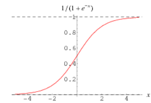
As the name “Logistic”, makes us think that there might be a function known as Logistic which is involved in the hypothesis of the Machine Learning Algorithm. Is our thinking in the right direction? Yes, it is!!! The Sigmoid Function is alternatively known as Logistic Function also.

f(x) is the Sigmoid Function

Now, moving on to the hypothesis of Logistic Regression:

theta_1, theta_2, theta_3 , …., theta_n are the parameters of Logistic Regression

Let’s have a look at the graph of Sigmoid Function:

Sigmoid Function’s Graph

So, the output of the Sigmoid Function ranges from 0 to 1. But for classification, a particular label should be predicted that indicates a class. In that case, a threshold (obviously a value between 0 and 1) needs to be set in such a way that it fetches the maximum predictive performance (performance analysis is discussed in the later part of the article).

Naturally, when there is a hypothesis, there is surely a Cost Function involved also.

This Cost Function is also known as Binary Cross Entropy Function.

Here, this cost function has to be minimized. Hence, minima (theta_0, theta_1, theta_2, … , theta_n) needs to be found.

Batch Gradient Descent can be used as an Optimization Technique to find this minima.

The implementation of Logistic Regression is done by creating 3 modules.

=>hypothesis(): It is the function that finds the output of the hypothesis of the Algorithm, given the theta (list of theta_0, theta_1, theta_2,…,theta_n), feature set X and number of features n. The implementation of hypothesis() is given below:

def hypothesis(theta, X, n):    h = np.ones((X.shape[0],1))    theta = theta.reshape(1,n+1)    for i in range(0,X.shape[0]):        h[i] = 1 / (1 + exp(-float(np.matmul(theta, X[i]))))    h = h.reshape(X.shape[0])    return h

=>BGD(): Here, the Gradient Descent Algorithm is implemented. It returns theta (list of theta_0, theta_1, theta_2, …, theta_n) that forms the minima, theta_history (contains the values of theta for every iteration) and cost (contains the value of cost function at every iteration), given initial theta (list of theta_0, theta_1, theta_2, … , theta_n), alpha (learning rate), num_iters (number of iterations), h (hypothesis value for all samples), Feature Set X, Label Set y and number of features n. The implementation of BGD() is given below:

def BGD(theta, alpha, num_iters, h, X, y, n):    theta_history = np.ones((num_iters,n+1))    cost = np.ones(num_iters)    for i in range(0,num_iters):        theta[0] = theta[0] - (alpha/X.shape[0]) * sum(h - y)        for j in range(1,n+1):            theta[j]=theta[j]-(alpha/X.shape[0])*sum((h-y)                               *X.transpose()[j])        theta_history[i] = theta        h = hypothesis(theta, X, n)        cost[i]=(-1/X.shape[0])*sum(y*np.log(h)+(1-y)*np.log(1 - h))    theta = theta.reshape(1,n+1)    return theta, theta_history, cost

=>logistic_regression(): It is the main function that takes the Feature Set X, Label Set y, learning rate alpha and number of iterations (num_iters). The implementation of logistic_regression() is given below:

def logistic_regression(X, y, alpha, num_iters):    n = X.shape[1]    one_column = np.ones((X.shape[0],1))    X = np.concatenate((one_column, X), axis = 1)    # initializing the parameter vector...    theta = np.zeros(n+1)    # hypothesis calculation....    h = hypothesis(theta, X, n)    # returning the optimized parameters by Gradient Descent...    theta,theta_history,cost = BGD(theta,alpha,num_iters,h,X,y,n)    return theta, theta_history, cost

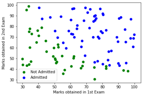
Going to the Application Part of the Article on a Practical Practice Dataset. The Dataset contains marks obtained by 100 students in 2 exams and the label (0/1), that indicates whether the student will be admitted to a university (1 or negative) or not (0 or positive). The Dataset is available at

navoneel1092283/logistic_regression

Problem Statement: “Given the marks obtained in 2 exams, predict whether the student will be admitted to the university or not using Logistic Regression”

Data Reading into Numpy Arrays :

data = np.loadtxt('dataset.txt', delimiter=',')X_train = data[:,[0,1]] # feature-sety_train = data[:,2] # label-set

Scatter Plot Visualization of the Dataset:

x0 = np.ones((np.array([x for x in y_train if x == 0]).shape[0],               X_train.shape[1]))x1 = np.ones((np.array([x for x in y_train if x == 1]).shape[0],               X_train.shape[1]))#x0 and x1 are matrices containing +ve and -ve examples from the#dataset, initialized to 1

k0 = k1 = 0

for i in range(0,y_train.shape[0]):    if y_train[i] == 0:        x0[k0] = X_train[i]        k0 = k0 + 1    else:        x1[k1] = X_train[i]        k1 = k1 + 1

X = [x0, x1]colors = ["green", "blue"] # 2 distinct colours for 2 classes 

import matplotlib.pyplot as pltfor x, c in zip(X, colors):    if c == "green":        plt.scatter(x[:,0],x[:,1],color = c,label = "Not Admitted")    else:        plt.scatter(x[:,0], x[:,1], color = c, label = "Admitted")plt.xlabel("Marks obtained in 1st Exam")plt.ylabel("Marks obtained in 2nd Exam")plt.legend()

Scatter Plot Visualization

Running the 3-module-Logistic Regression:

# calling the principal function with learning_rate = 0.001 and # num_iters = 100000theta,theta_history,cost=logistic_regression(X_train,y_train,0.001)

The theta output comes out to be:

theta after BGD for Logistic Regression

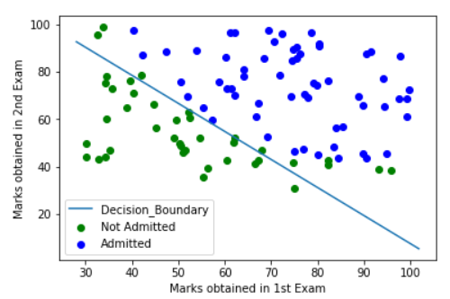
This Visualization of theta obtained can be done by incorporating the Decision Boundary (theta based separating line between 2 classes) in the Scatter Plot:

plot_x = np.array([min(X_train[:,0]) - 2, max(X_train[:,0]) + 2])plot_y = (-1/theta[2]) * (theta[1] * plot_x + theta[0])

for x, c in zip(X, colors):    if c == "green":        plt.scatter(x[:,0],x[:,1],color = c, label = "Not Admitted")    else:        plt.scatter(x[:,0], x[:,1], color = c, label = "Admitted")plt.plot(plot_x, plot_y, label = "Decision_Boundary")plt.legend()plt.xlabel("Marks obtained in 1st Exam")plt.ylabel("Marks obtained in 2nd Exam")

The Decision Boundary incorporated Scatter Plot looks like:

The gradual reduction in Cost Function is also visualized using Line Plot:

import matplotlib.pyplot as pltcost = list(cost)n_iterations = [x for x in range(1,100001)]plt.plot(n_iterations, cost)plt.xlabel('No. of iterations')plt.ylabel('Cost')

The Line-Curve turns out to be:

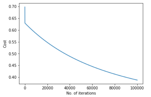Line Curve Representation of Cost Minimization using BGD for Logistic Regression

Model Performance Analysis:

In classification, model performance analysis is done on the following metrics:

Getting the predictions…

X_train = np.concatenate((np.ones((X_train.shape[0],1)), X_train)                          , axis = 1)h = hypothesis(theta, X_train, X_train.shape[1] - 1)# Taking 0.5 as threshold:for i in range(0, h.shape[0]):    if h[i] > 0.5:        h[i] = 1    else:        h[i] = 0

=>Accuracy: Ratio of no. of correctly predicted samples to total no. of samples.

Finding Accuracy:

k = 0for i in range(0, h.shape[0]):    if h[i] == y_train[i]:        k = k + 1accuracy = k/y_train.shape[0]

The output of accuracy comes out to be:

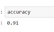Output of Accuracy => 91% Accuracy

=>Precision: Ratio of no. of correctly predicted positive observations to the total no. of predicted positive observations.

Finding Precision:

tp = fp = 0# tp -> True Positive, fp -> False Positivefor i in range(0, h.shape[0]):    if h[i] == y_train[i] == 0:        tp = tp + 1    elif h[i] == 0 and y_train[i] == 1:        fp = fp + 1precision = tp/(tp + fp)

Output of Precision

=>Recall: Proportion of correctly identified positives.

Finding Recall:

fn = 0# fn -> False Negativesfor i in range(0, h.shape[0]):    if h[i] == 1 and y_train[i] == 0:        fn = fn + 1recall = tp/(tp + fn)

Output of Recall

=>F1-Score: Harmonic Mean of Precision and Recall

Finding F1-Score:

f1_score = (2 * precision * recall)/(precision + recall)

Output of F1-Score

Confusion Matrix:

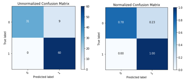
Structure of Confusion Matrix

tn = 0# tn -> True Negativefor i in range(0, h.shape[0]):    if h[i] == y_train[i] == 1        tn = tn + 1

cm = np.array([[tp, fn], [fp, tn]])

# MODULE FOR CONFUSION MATRIX

import matplotlib.pyplot as plt%matplotlib inlineimport numpy as npimport itertoolsdef plot_confusion_matrix(cm, classes,                          normalize=False,                          title='Confusion matrix',                          cmap=plt.cm.Blues):    """    This function prints and plots the confusion matrix.    Normalization can be applied by setting `normalize=True`.    """    if normalize:        cm = cm.astype('float') / cm.sum(axis=1)[:, np.newaxis]        print("Normalized confusion matrix")    else:        print('Confusion matrix, without normalization')

print(cm)

plt.imshow(cm, interpolation='nearest', cmap=cmap)    plt.title(title)    plt.colorbar()    tick_marks = np.arange(len(classes))    plt.xticks(tick_marks, classes, rotation=45)    plt.yticks(tick_marks, classes)

fmt = '.2f' if normalize else 'd'    thresh = cm.max() / 2.    for i, j in itertools.product(range(cm.shape[0]), range(cm.shape[1])):        plt.text(j, i, format(cm[i, j], fmt),                 horizontalalignment="center",                 color="white" if cm[i, j] > thresh else "black")

plt.tight_layout()    plt.ylabel('True label')    plt.xlabel('Predicted label')

plt.figure()# Un-Normalized Confusion Matrix...plot_confusion_matrix(cm, classes=[0,1], normalize=False,                      title='Unnormalized Confusion Matrix')# Normalized Confusion Matrix...plot_confusion_matrix(cm, classes=[0,1], normalize=True,                      title='Normalized Confusion Matrix')

The above example is actually an application of Binary Classification. To tackle Multi-Class Classification Problems, the strategy of Binary Classification can be repeated N no. of times where N is the number of classes using the concept of One Vs. Rest, which results in an ensemble model containing N sub-models.

Future Scope

The future scope for the readers involve application of other advanced optimization techniques other than Gradient Descent which does not require learning rate to be given as input but, is able to accurately or roughly find the Global Minima of the Cost Function (theta).

That’s all regarding Logistic Regression in Python from scratch.

For Personal Contacts regarding the article or discussions on Machine Learning/Data Mining or any department of Data Science, feel free to reach out to me on LinkedIn

Navoneel Chakrabarty - Founder - Road To Financial Data Science | LinkedIn

Logistic Regression in Python from scratch was originally published in Hacker Noon on Medium, where people are continuing the conversation by highlighting and responding to this story.