Dynamic Models and Simulation

An overview of simulation techniques and applications, with a description of an exciting theory you might not be familiar with.Galactic filaments take shape in a trillion-particle cosmological simulation. Credit: Dark Sky Simulations Collaboration

In the prior article it was observed that a model is a simplified representation of some aspect of reality — the target system — and a dynamic model is one that incorporates the laws that govern how the target system changes in time. Simulation, then, is the act of running a dynamic model.

To perform a simulation, we set up the model’s initial state, set it in motion, and observe its progression. Crucially, a simulation can be made interactive by providing a means for one or more persons to act upon the model as it runs, thereby altering its progression. In this way, human actors can serve as components of the model.

As with models in general, simulations can be divided into three categories by purpose — scientific, utilitarian, or experiential.

The purpose of scientific simulation is to understand and explain natural processes such as the behavior of molecules, the formation of galaxies, or the origins of economic downturns. It provides a way to perform virtual experiments on systems that cannot be acted upon directly.

Scientific simulations often model generic systems rather than particular ones. For example, a simulated galaxy need not represent an actual observed galaxy to provide insight into why, say, some galaxies develop spiral arms.

The purpose of utilitarian simulation is to assist real-world interactions with the target system. There are two broad categories: simulation used for prediction and simulation used for training.

When a simulation models a particular real-world system (as opposed to a generic one), its progression amounts to a prediction of how the real-world system will itself progress. Some systems, such as the solar system, can be accurately simulated millions of years into the future. Others, such as the weather, are much more difficult to predict because they are chaotic, meaning that the way they progress is critically dependent on their initial conditions, which can only be modeled approximately.

Since simulation can predict the evolution of a system, it follows that it can also predict the effects of an intervention on that system. Simulation can thus assist in the planning of interventions. For example, an intervention intended to reduce the amount of carbon dioxide in the atmosphere can be tested in simulation before it is attempted in reality.

Simulation can also assist in the design of engineered systems, and this too is a variety of prediction. In this case, we use simulation to predict, for example, whether a building will collapse in an earthquake, whether a circuit will operate as intended, and so on. Such simulations are unique in that, although the target system is a particular system, it is a system that does not yet exist.

Interactive simulations provide a kind of artificial experience and are thus useful for training. Training simulations offer a risk-free way to gain experience with complicated systems such as vehicles, battlefields, and business environments.

Lastly, the purpose of experiential simulation is to provide an audience with an experience that is valuable in its own right, regardless of its real-world utility. Although it might be interesting to passively observe a simulation as it unfolds, most experiential simulations are interactive — they are games, in other words.

Experiential simulations typically model generic systems because they do not need to make predictions, and they are often stylized, or non-realistic, because they do not need to aid real-world activities (though nothing prevents them from doing either of these things). Their target systems range from abstract, such as the combinatoric principles modeled by a card game, to concrete, such as the physical environments modeled by many computer games.

Computer Simulation

A physical model is one that is comprised of physical materials such as wood or plastic, and physical simulation is the act of setting a physical model in motion. This might entail switching on a fan, opening a valve, or blowing a whistle. In computer simulation, by contrast, the model is built from symbols — numbers stored in memory — and a computer program updates the symbols from one time-step to the next.

As an example, consider the problem of calculating how far an artillery shell will travel given the firing angle of the gun, the initial velocity of the shell, and the atmospheric conditions. Although there are equations that accurately describe the motion of a projectile through the air, they have no “analytical solution”. That is to say, there is no formula that will give us the distance traveled just by plugging in the firing angle and other parameters. Instead, we must resort to “numerical integration” — we must advance the shell along its path in small time-steps, updating its position and velocity at every step. When the simulated shell hits the ground — i.e., when the memory location representing its altitude goes negative — we have our answer.

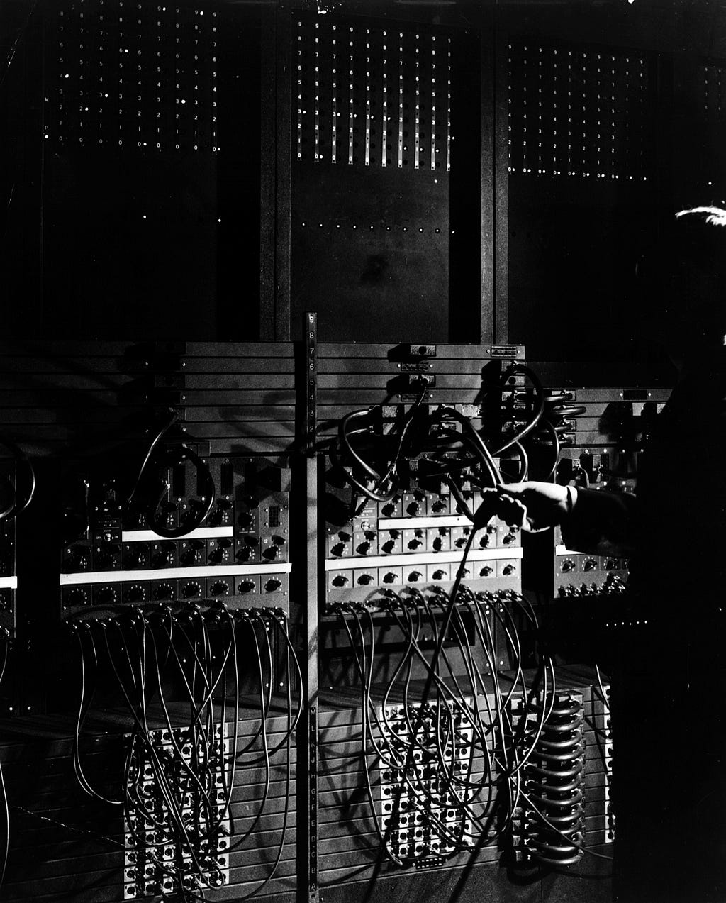
The first general-purpose computer, ENIAC (Electronic Numerical Integrator and Computer), was commissioned by the US Army to perform exactly this kind of ballistic simulation. The machine was completed in 1945 — too late to contribute to the war effort — but by then its versatility and exceptional speed had attracted the attention of scientists at Los Alamos, who used it to run a simulation to test the feasibility of a hydrogen bomb. (They were impressed enough to build their own similar computer — the Mathematical and Numerical Integrator and Computer, or MANIAC.) The Los Alamos scientists were interested not in the motions of artillery shells but of neutrons, and ENIAC’s programmability meant that it could be reconfigured for this purpose.

ENIAC was programmed by setting switches and plugging in cables. Credit: US Army Research Laboratory

Like the numerous computers it inspired, ENIAC was, fundamentally, a simulation machine. To this day, the most distinguishing aspect of computers remains this ability to breathe life into dynamic models. Modern simulations are far more detailed than the ones ENIAC ran, but the core idea is unchanged: values analogous to real-world quantities and attributes are stored in memory and updated from one time-step to the next.

Computer Simulation Techniques

The first consideration when programming a computer simulation is how to advance the time. It is not known for certain whether time is discrete (meaning that it advances in small increments) or continuous (meaning that it is infinitely divisible into ever smaller segments). Either way, nature’s time-steps are inconceivably tiny. It follows that a programmer should select time-steps that are small enough to ensure accuracy (assuming that’s the goal), yet large enough to ensure that a result can be obtained in a reasonable amount of (real) time.

The simplest approach is to settle on a fixed-length time-step that will apply throughout the simulation. It’s often more efficient, though, to implement adaptive time-steps, where the steps are shorter in regions of the simulation where things are unfolding quickly or where forces are strong, but longer in regions where relatively little is happening.

Discrete event simulation is a technique that takes the idea of adaptive time-steps to its logical endpoint. In this approach, we calculate when the next “event” (however we define it) will occur and advance the clock directly to that event. As an example, consider a simulation of customers lining up at a supermarket checkout. It is much more efficient to calculate the amount of time each customer will take to complete their transaction, and how much time will elapse before the next customer arrives in line, than it is to continually step through time waiting for these events to occur. Furthermore, the event-times can be specified with as much precision as memory allows; there is no need to fit them to arbitrary step sizes.

Discrete event simulation is less helpful in simulations involving forces such as gravity, since a force is felt at every infinitesimal point in time — like a continuous, ongoing event. In such cases, stepping is required. Collisions between objects, by comparison, do qualify as discrete events.

There is obviously a large degree of uncertainty involved in calculating how long a customer will spend at the cash register and how long it will take for the next customer to arrive in line. Since there is no way to predict these time-spans (short of simulating the lives and minds of every potential customer), they must be generated randomly. Our supermarket simulation would thus be non-deterministic, or stochastic.

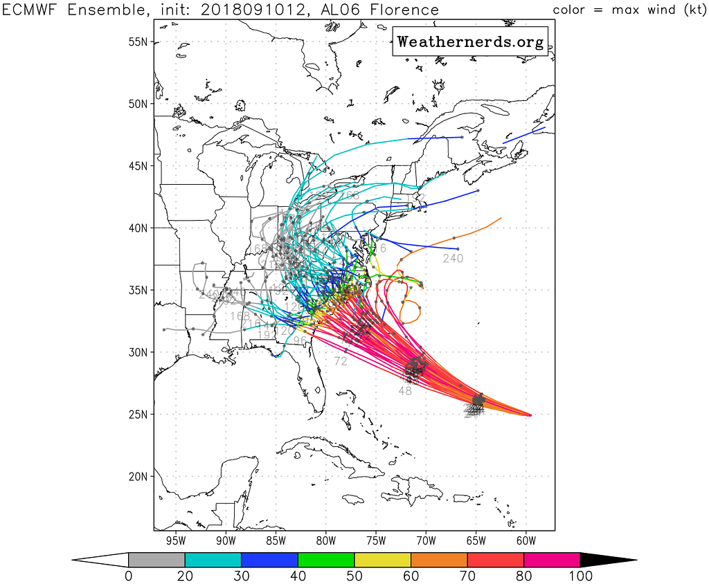
In stochastic simulation, a degree of randomness influences how the simulation progresses. One way that randomness can be helpful stems from the fact that no simulation is ever perfectly accurate, and that we can manage this inaccuracy by running the same simulation many times. The outcomes will vary (thanks to the randomness), allowing us to identify a range of possible outcomes. Furthermore, we can estimate the probability of a given outcome just by counting the number of times it occurs. Of course, the quality of such an estimate depends on the realism of the simulation and its stochastic processes.

A plot of the outcomes of multiple stochastic simulations to predict the path of Hurricane Florence. Credit: weathernerds.org

This technique — running a stochastic simulation many times and tallying the results — is called Monte Carlo simulation. Its use was pioneered by the same scientists who commandeered the ENIAC for their nuclear research; the simulations they ran were the first to use the Monte Carlo method.

More recently, a variation of the technique called Monte Carlo Tree Search has been applied to turn-based games such as Go and Chess. The idea is to run very many simulations of a game from the current board position to the end, keeping a tally of simulated wins and losses to estimate the best move.

The ballistic simulation described previously depicts the behavior of a single body (the artillery shell), but a simulation can incorporate as many bodies as computing resources allow. An N-body simulation (or particle-based simulation) consists of a number of particles located in space along with equations that govern how the particles move and interact.

A particle-based simulation of the debris disk surrounding a star. Credit: NASA’s Goddard Space Flight Center

The canonical example is a gravitational simulation, where in each time-step the program 1) calculates the force of gravity acting between every pair of particles; 2) updates each particle’s velocity according to the net force acting on it; and 3) updates each particle’s position according to its velocity.

This algorithm can be optimized (sped up) by a technique described as a tree code, which identifies clusters of particles that can be treated as single particles with respect to other, distant particles.

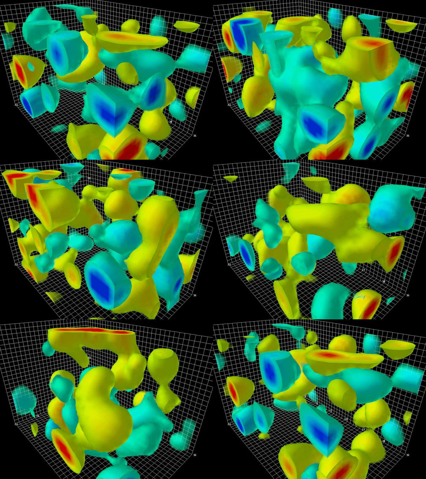
While a particle-based simulation stores values for each particle (its position, velocity, and other attributes), a field-based simulation works by partitioning space into a grid of cells and storing values for each cell.

A field-based simulation of quantum field fluctuations in a vacuum. Credit: Derek Leinweber

In a simulation of a fluid, for example, the cells contain values representing the fluid’s density, temperature, pressure, and so on, and hydrodynamic equations govern how the values change from one time-step to the next.

Field-based simulations can be optimized by a technique called adaptive mesh refinement, where cells are automatically subdivided into smaller cells in regions that are particularly active.

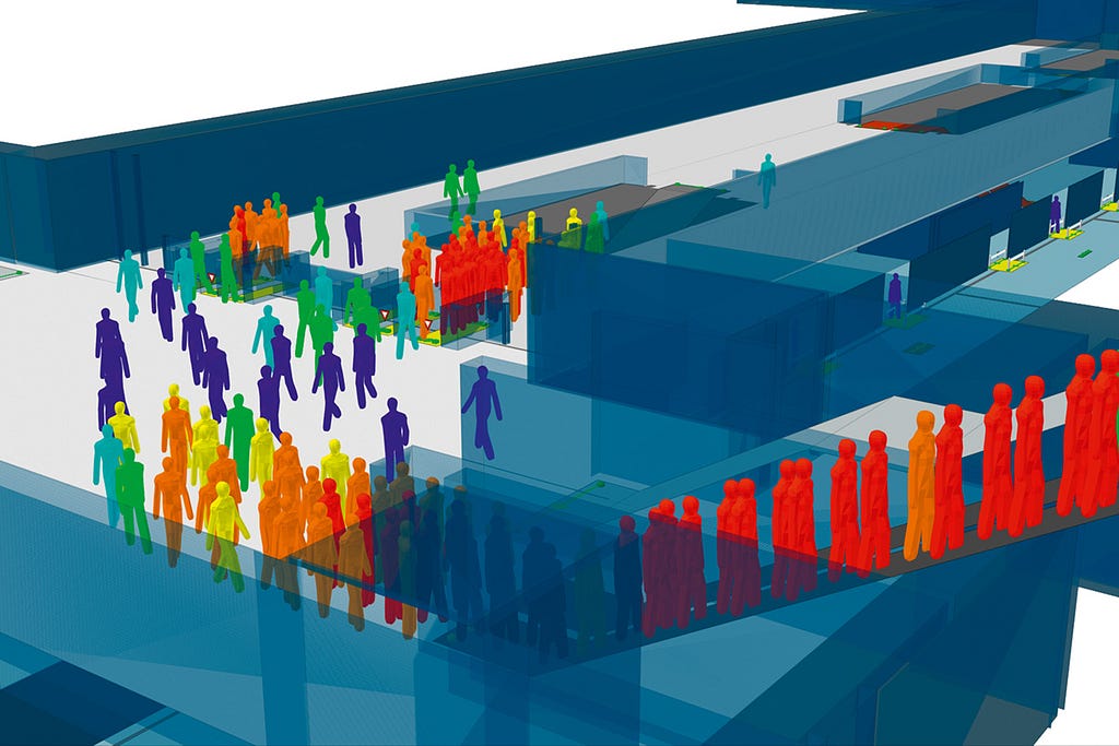
While particle- and field-based simulations are useful for modeling inanimate matter and energy, an agent-based simulation consists of a number of autonomous agents acting within an environment. The agents are governed not by global equations but by their own internal programs. They observe their local surroundings, process their observations, and decide what actions to take next.

Agents that select their actions according to a fixed set of if/then rules are described as reactive, since they are unable to formulate proactive plans. Agents that employ more capable techniques, such as neural networks, are described as cognitive. Agents with changeable internal states are said to possess memory (however tiny it may be), and changes to those internal states constitute learning. If an agent shares its internal state with other agents, it is said to communicate.

It is apparent that an agent’s internal program can be implemented in countless ways. In fact, by a growing consensus the field of artificial intelligence is the study of intelligent agents, and the numerous techniques and algorithms employed in that discipline can be applied equally well in simulation.

An agent-based simulation to analyze the flow of pedestrians through a proposed transit hub. Credit: Oasys SoftwareSimulation and Cognition

Simulation provides a means of predicting the future. This is not only useful in its own right (when predicting the weather for example), but it is also the basis of a further capability — simulation can be used to guide the actions of an autonomous agent.

As we have seen, Monte Carlo Tree Search (MCTS) operates in this way. In MCTS, many simulations of a game are run from the current position to the end, and a tally is kept of simulated wins and losses to identify the best move. This procedure can be viewed as a kind of agent-based simulation with two competing agents — the opponent-agent and the self-agent — serving as models of the actual players. The primary agent “thinks” by observing the outcomes of the matches between the simulated players. This approach is especially effective when a neural network is used to model the players. (This is the method employed by the game-playing program AlphaZero, which will be described in a future article.)

MCTS can be applied to any game where time advances in discrete turns and where a finite (preferably small) number of discrete moves is available at every turn. But what about agents that operate in continuous, real-time environments, such as self-driving cars, self-landing rockets, and acrobatic robots?

This is the domain of control theory, which is the study of the automated control of machinery. A simple example is a car’s cruise control, which senses the car’s speed, compares it to the desired speed, and calculates a new throttle setting to reduce the difference. This process continues in a perpetual feedback loop, continually recalculating the throttle setting so long as the cruise control remains engaged.

One method of control in particular, Model Predictive Control (MPC), has proven effective for agents that are difficult to control because of their complicated dynamics. MPC works by performing many simulations of the agent’s motions in its environment, starting from the present moment and continuing for a certain number of time-steps into the future (the so-called prediction horizon). In each simulation, a different sequence of control actions is assumed; these might be changes to the position of a steering wheel, the operation of actuators, and so on. When a simulation is completed, the control sequence is scored according to some scheme devised by the engineers. For example, if a simulated vehicle drifts off course, or collides with something, or tips over, then the control sequence will score poorly. Finally, once the real-world time has advanced by the equivalent of one simulated time-step, the highest-scoring control sequence is identified, and the first action in that sequence is executed (the subsequent actions are ignored since a new sequence will be computed in the next time-step).

Clearly, this algorithm is very similar to MCTS. Indeed, if an MPC model incorporates stochastic elements — perhaps in the form of random gusts of wind, or in the behaviors of other agents — then it is effectively Monte Carlo simulation. For both MPC and MCTS, the guiding principle is the same — an agent simulates itself performing the actions it is considering. The simulation may or may not incorporate other agents (such as the opponent-agent in MCTS), and it may be continuous (MPC) or discrete (MCTS).

In the field of cognitive neuroscience, there is convincing evidence that the brain follows this same principle. The simulation theory of cognition proposes that the regions of the brain that control the muscles and process sensory data are invoked not just for real-world actions and perceptions, but for imaginary ones as well.

The idea is this: An imaginary action is orchestrated in the motor cortex in the same way as an ordinary one, except that the final output to the muscles is inhibited. This imagined action, in conjunction with related memories, evokes sensory data representing how the action is likely to unfold. This data is processed by the sensory cortex like real sensory data — perhaps leading to the next imaginary action. It is thought that this process applies not just to simple motor activity, but to thinking in general — imagining scenarios, considering hypotheticals, forming long-term plans, and so on. It is reasonable to suspect that it might apply to dreaming as well.

An enticing aspect of this idea of cognition-by-simulation is that it offers a plausible means by which consciousness might arise. Simulation provides the artificial experiences that comprise a conscious agent’s “inner world”, while it simultaneously reveals the potential futures an agent might bring about through its actions, which could manifest as an impression of free will.

There is likely a third ingredient that’s needed for consciousness to emerge: the continual elaboration and refinement of the dynamic models upon which the simulations are based. In a word, learning. In biological brains, models take the form of memories, such as the muscle-memories that guide simple actions or the explicit memories that guide more deliberative activities. As a biological agent interacts with its environment, new memories are continually accumulated and integrated with existing ones in a way that is baked into the control loop. Precisely how this works is not well understood, but this much is certain: whenever an action unfolds in a way that was not anticipated, there is something to be learned.

Unlike biological memory, the models used in MCTS and MPC are typically pre-designed by engineers and thus fixed. But progress has been made in making these techniques more adaptive — and generally more capable — by incorporating machine learning. AlphaZero, as mentioned previously, uses a neural network to model the simulated player-agents (i.e. to select their simulated moves). This network is trained through self-play — it learns solely through direct experience within the environment that is the game. Another example comes from the realm of control engineering, where robots are being built that can improve their models — and hence their dexterity — by interacting and experimenting with their environments, much like children playing.

In both these examples, the agents are trained by reinforcement learning, a type of machine learning that has striking corollaries to learning in biological brains. This simple yet powerful learning procedure will be the topic of a future article.

TLDR: Simulation is the act of stepping a dynamic model forward in time. Simulation can be used to study inaccessible systems, to provide artificial interactive experiences, and to predict the future. An autonomous agent can predict the consequences of its actions — and thus decide how best to act — by simulating itself performing the actions it is considering. There is strong evidence that biological brains work in this way, and there are hints that this process of interactively simulating oneself into the future might facilitate the emergence of consciousness.

Thanks for the read! Please have a look at my game Thetaball on Steam — it’s the first application of an experimental game engine I’m developing for evolving intelligent agents in physics-based environments.

Dynamic Models and Simulation was originally published in Hacker Noon on Medium, where people are continuing the conversation by highlighting and responding to this story.