More price functions for Token-Bonding Curves

Following last week’s article, written by Alexandre Pinto, the author of Arrays in Solidity and Working with Strings in Solidity, today we continue talking about the Token Bonding Curves.

In my previous post about Token-Bonding Curves, I showed that Bancor only allows 4 different types of curves. But that does not have to be the whole story, if we allow the reserve ratio to fluctuate. Today, I examine some variants that don’t fit in that scheme.

Positive Initial price

I start with simple variants of the Bancor’s curves. The Bancor price curves can all be represented by a function of form

where k can be any real value and C ≠0.

This function always goes through the origin of the graph, that is, the price of a token at supply 0 is also 0.

An easy change is to make this a positive price:

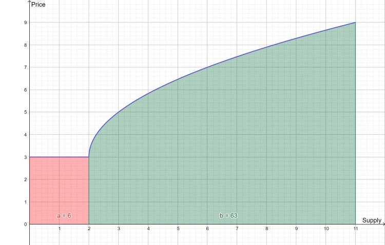
The above graph shows one such curve,

where a standard curve has been pushed up from the x-axis by 6 units. It is still easy to integrate:

We can use this to compute the reserve for the two points market in the graph:

The corresponding market caps are 108 and 27. It is easy to conclude the reserve ratio is not constant. One way to look at this is that we have an extra rectangle added to an area with a constant reserve ratio. As the supply grows, the relative importance of the lower rectangle’s area diminishes as the area of the rest of the curve increases. That means the reserve ratio is very high for low supplies, but will decrease as the supply grows.

There is a lower limit for this ratio, and we can deduce it intuitively. Fix a point X that we want to compute this ratio for, and let the price curve be

There are two parts to the area under the curve: one is the area under the horizontal that represents the initial price (area A); the other is the area between this horizontal and the curve (area B). The market cap, on its turn, includes area A again, and everything between this and the horizontal line that passes through X. If area A were 0, (ie the initial price would be 0) then the reserve ratio would be k. When it is not, area A contributes both to the reserve and the market cap, and so the reserve ratio can only increase. This means that this kind of curve, with a non-null initial price, guarantees that the reserve ratio is at least what the constant ratio would be with a null initial price.

This comes at the expense of higher prices for users, who in each trade have to pay a fixed contribution to this excess of reserve.

Reserved Supply

Another variant of the standard curves is one in which the market owner reserves some supply that cannot be traded. This makes more sense in a minting curve (one that creates the tokens when they are sold) than in a deposit curve (one which only transfers existing tokens from its own address to the user’s wallet). In one scenario, these reserved tokens do not affect the curve’s price, and the result is simply that it’s as if they did not exist. In a deposit bonding curve, it’s as good as if these had never been deposited in the curve in the first place.

The formula for these curves is:

As written, this curve would have the same behaviour to the left of

as it has to the right. The only effect of shifting the curve like this is fix a different value for the price of the first token (this is a more complicated way of achieving the same behaviour of the previous section). But it becomes more interesting if we introduce a change of function at point

and instead define, say, a horizontal function between 0 and

The best way to do that is even to join both variants, and write a price function like this:

In this situation, the market owner decides to start a Market but reserves the first batch of tokens at a different price: this could be constant; follow a different curve; or even the tokens could be declared as non- tradable, and the price function simply would not be defined in this range. It also sets a minimum price for all future tokens, thus guaranteeing a minimum reward for the owners of the reserved supply who wish to sell their tokens to the curve. And of course, this curve also guarantees a minimum reserve ratio of k.

The reserve itself now has to be calculated in two parts, one for each branch of the function, but aside from that, there is nothing mathematically new in this function. The formula for the reserve is this:

Quasi-polynomial function types

The polynomial functions examined in the post referred previously do not exhaust all the capabilities. If we relax the fixed reserve requirement, we could experiment with other functions. A good way to choose a function is to think a priori of the behaviour and incentives we want to enforce in the market, and then see how to model them. We can see an example of this in this post by Wilson Lau, where the following function is derived (in general terms):

Despite the logarithm in the exponent, this can still be rewritten as

for

which falls exactly in the previous case of the reserved supply.

But there is also a second formula that is another kettle of fish, and introduces a whole new shape:

There are 5 different parameters here, which complicate things a little. We can rewrite the above like this:

which is not an immediate improvement but clarifies something: the dominant term here is of the form

which, once it turns positive, is a function that grows extremely slow. For reference, it turns 1 for

it is 2 for

and it turns 3 for

Given this rate of growth, for most practical applications it can probably be considered a constant, which places the above price formula in the company of a more boring class of function like

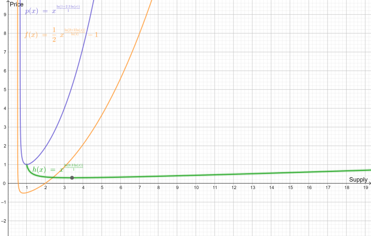
But this happens only after x turns smooth. It is a wholly different affair for small values of x, where the price function plunges almost vertically (depending on the choice of constants), until turning around and emulating a simple power function. This initial drop in value may not be suitable for normal market incentives, so study your curve well before implementing one, and in particular have an idea of the maximum and minimum range of supply the market is going to work. Here is an example of 3 curves of this type:

Exponential Functions

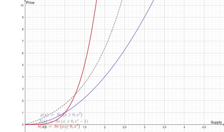
The last example introduced the possibility of using the variable in the exponent (albeit tempered by a double logarithm function). This opens the door to the simple but dramatic exponential function. On the surface, its graph is similar to power functions of exponent larger than 1 and for positive variable. When the variable is negative, these functions are radically different: the exponential function will seem to hug the horizontal axis, being almost a horizontal line, but the power functions will be a symmetric of the positive side of the graph: if the exponent’s numerator is even, it will be symmetric around the y-axis; if it is odd, it will be symmetric around the origin point. Another difference is that the power functions pass through the origin of the chart, and a vanilla exponential function does not. But with a little tweaking, we can write an exponential that does, eg:

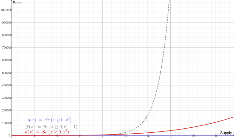
Despite the similarities, the exponential function is NOT like a power function: it grows much, much faster than any polynomial function (for large enough x). An example of this is in the next figure, that shows the exact same functions as above for modest, but larger, values of supply (up to 20). See how the exponential function takes off in relation to the others.

The exponential function has a very simple integral, and we can easily check that it does not produce a constant ratio. Below, I list a generic exponential price function, the corresponding reserve and the calculation of the reserve ratio.

The reserve ratio is

which shows this varies with the supply, and so is not constant.

Logarithmic Functions

The logarithmic function is like the mirror of the exponential function. While the exponential function grows very fast and approximates a vertical curve, the logarithmic function grows very slowly, and instead approximates a horizontal.

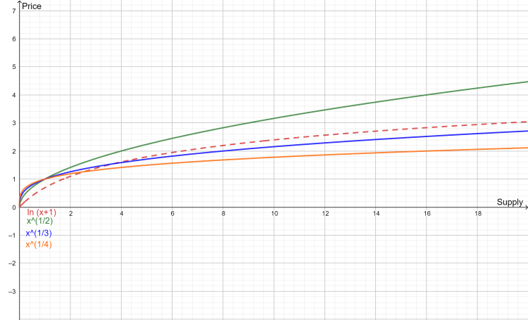
The next figure shows a comparison of the logarithmic function with power functions of exponents

Their approximate shapes are similar, and one could think the logarithmic function (in a dashed line) to be just of the same type as the power functions. It does overtake two of the others, and from this small example it looks like it could dominate them. However, this is short lived behaviour. The truth is that as S tends to infinity, the logarithmic function grows slower and slower and slower, until it is overtaken by all other power functions.

The graph below shows the same functions in the vicinity of S= 90000 where the log function is already the smallest of the bunch.

The integral of

is more complicated than the previous ones:

Potential drawbacks of this function include the necessity to implement a logarithmic function, since this is not available in solidity off the shelf. It also is not easy to generalise the above function itself by increasing the degree of

to

which includes a trigonometric function in the integral. Higher exponents don’t even have a closed integral formula.

Negative Exponential

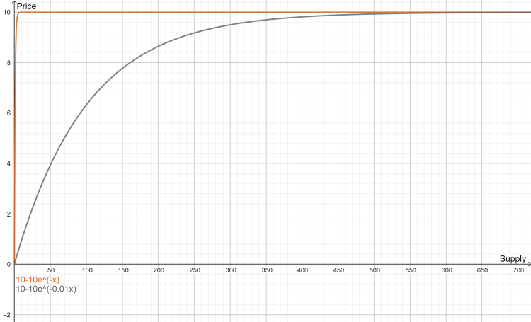
An interesting alternative to the logarithm function may be the negative exponential. Unlike the logarithm, which grows indefinitely and tends to infinitely (albeit at a very slow pace), the negative exponential has a true horizontal asymptote, meaning that it will approximate a true horizontal function and never go over a limit value. For example:

approximates the maximum value C. The rise of the function is steep for

and the passage to the near-horizontal regime is almost abrupt. To make the rise softer, we can make a much smaller, as long as it is still positive.

The integral (and therefore the reserve) is not complicated:

Here is an example graph:

Conclusion

In this long post, I have gone over several possible price functions for Token-Bonding Curves (TBC), and talked a little about their properties and how to compute their integral. The choice of function should primarily be dictated by the desired incentive, possibly by sketching a chart with the desired behaviour and then identifying a function close to it.

Importantly, any choice must then be validated according to the ease or difficulty of implementing the necessary functions. In a TBC, we want both to sell and buy tokens from the curve. We only need to compute the integral of the price function if we want to sell or buy a given number of tokens, but if we want to buy or sell tokens equivalent to a given amount of the reserve currency, then we need the inverse function of this integral.

To ease on the maths (which is already rather heavy) I have not given any of these inverse functions. This is a bigger challenge than it seems on the surface. For example, the inverse of the reserve for a function in the section “Positive initial price” would involve solving a polynomial equation of the kind

which for high values of k is not straightforward.

The exponential functions would not pose much of a problem, nor would the simpler function in “Quasi-polynomial function types”. The second kind in this section, however, would be very hard to solve analytically for both the reserve and its inverse. This also applies to the inverse of the reserve for a logarithmic function. Finally, even the negative exponential reserve is not easy to invert.

This makes it difficult to use most of the functions in this list in a TBC where we want to specify a currency value instead of the number of tokens to buy or sell (which is common in financial markets), but it is possible to provide a market that does not include the former. This is more similar to the material world, where many markets only work that way: we usually don’t buy 20$ worth of apples or meat, but rather look for a specified quantity or weight.

About the Author

Alex is a software engineer at Aventus, working on the blockchain engineering team. He has 20 years of experience working in technology, completing a PhD in Computer Science as well as a post-doctorate in Cryptography. As part of his research, Alex has published papers on Kolmogorov Complexity, Cryptography, Database Anonymization and Code Obfuscation.

Alex also spent seven years lecturing at the University Institute of Maia, including directing the degree programmes for BSc Computer Science and Information Systems and Software.

This article was originally posted on his blog.

More price functions for Token-Bonding Curves was originally published in Hacker Noon on Medium, where people are continuing the conversation by highlighting and responding to this story.