Non-Stationarity and Memory In Financial Markets

Stationarity and Memory in Financial Markets

Artistic impression of a multiverse. Credit: Jaime Salcido / EAGLE Collaboration

Stationarity and time series predictability, a special case of which is time series memory, are notions that are fundamental to the quantitative investment process. However, these are often misunderstood by practitioners and researchers alike, as attests Chapter 5 of the recent book Advances in Financial Machine Learning. I’ve had the pleasure to elucidate these misconceptions with some attendees of The Rise Of Machine Learning in Asset Management at Yale last week after the conference, but I’ve come to think that the problem is so widespread that it deserves a public discussion.

In this post I make a few poorly documented points about non-stationarity and memory in financial markets, some going against the econometrics orthodoxy. All arguments are backed by logic, maths, counter-examples and/or experiments with python code at the end.

The arguments made here can be divided into practical and technical arguments:

Technical Takeaways:

• It is impossible to test whether a time series is non-stationarity with a single path observed over a bounded time interval — no matter how long. Every statistical test of stationarity makes an additional assumption about the family of diffusions the underlying process belongs to. Thus, a null hypothesis rejection can either represent empirical evidence that the diffusion assumption is incorrect, or that the diffusion assumption is correct but the null hypothesis (e.g. the presence of a unit root) is false. The statistical test by itself is inconclusive about which scenario holds.
• Contrary to what is claimed in Advances in Financial Machine Learning, there is no “Stationarity vs. Memory Dilemma” (one has nothing to do with the other), and memory does not imply skewness or excess kurtosis.
• Iterated differentiation of a time series à la Box-Jenkins does not make a time series more stationary, it makes a time series more memoryless; a time series can be both memoryless and non-stationary.
• Crucially, non-stationarity but memoryless time series can easily trick (unit-root) stationarity tests.

The notions of memory and predictability of time series are tightly related, and we discussed the latter in our Yellow Paper. I’ll take this opportunity to share our approach to quantifying memory in time series.

Practical Takeaways:

• That markets (financial time series specifically) are non-stationary makes intuitive sense, but any attempt to prove it statistically is doomed to be flawed.
• Quantitative investment management needs stationarity, but not stationarity of financial time series, ‘stationarity’ or persistence of tradable patterns or alphas over (a long enough) time (horizon).

Stationarity

Simply put, stationarity is the property of things that do not change over time.

Quant Investment Managers Need Stationarity

At the core of every quantitative investment management endeavor is the assumption that there are patterns in markets that prevailed in the past, that will prevail in the future, and that one can use to make money in financial markets.

A successful search for those patterns, often referred to as alphas, and the expectation that they will persist over time, is typically required prior to deploying capital. Thus stationarity is a wishful assumption inherent to quantitative investment management.

Stationarity In Financial Markets Is Self-Destructive

However, alphas are often victim of their own success. The better an alpha, the more likely it will be copied by competitors over time, and therefore the more likely it is to fade over time. Hence, every predictive pattern is bound to be a temporary or transient regime. How long the regime will last depends on the rigor used in the alpha search, and the secrecy around its exploitation.

The ephemerality of alphas is well documented; see for instance Igor Tulchinsky’s latest book, The Unrules: Man, Machines and the Quest to Master Markets, which I highly recommend.

In regards to the widespread perception that financial markets are highly non-stationary though, non-stationarity is often meant in a mathematical sense and usually refers to financial time series.

Time Series Stationarity Can’t Be Disproved With One Finite Sample

In the case of time series (a.k.a. stochastic processes), stationarity has a precise meaning (as expected); in fact two.

A time series is said to be strongly stationary when all its properties are invariant by change of the origin of time, or time translation. A time series is said to be second-order stationary, or weakly stationary when its mean and auto-covariance functions are invariant by change of the origin of time, or time translation.

Intuitively, a stationary time series is a time series whose local properties are preserved over time. It is therefore not surprising that it has been a pivotal assumption in econometrics over the past few decades, so much so that it is often thought that practitioners ought to first make a time series stationary before doing any modeling, at least in the Box-Jenkins school of thought.

This is absurd for the simple reason that, (second order) stationarity, as a property, cannot be disproved from a single finite sample path. Yes, you read that right! Read on to understand why.

But before delving into an almost philosophical argument, let’s take a concrete example.

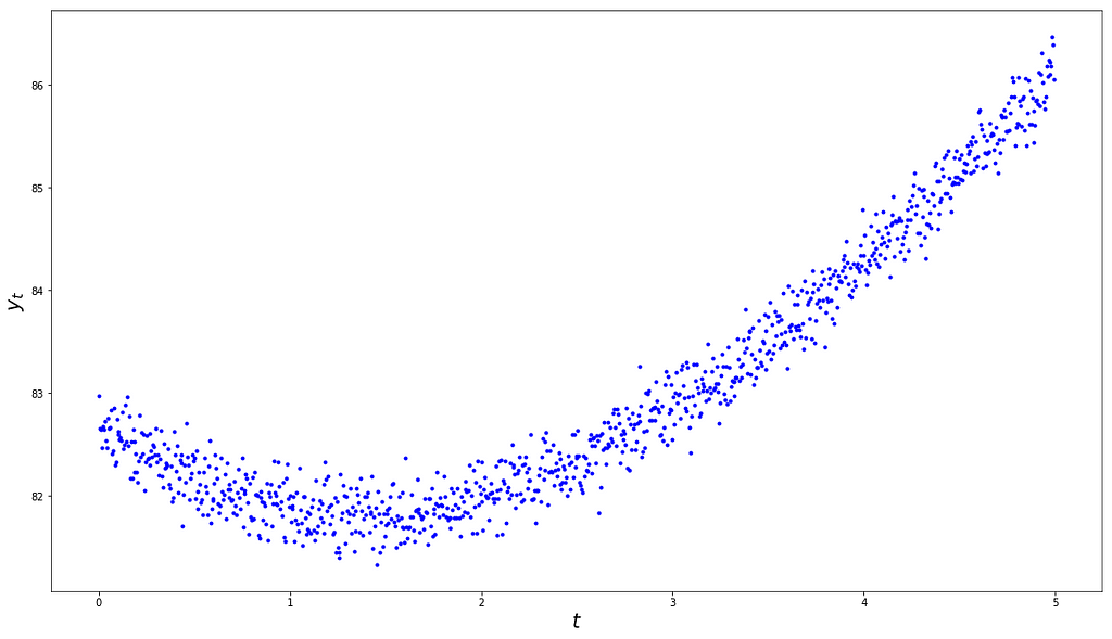Draw of a time series on a uniform grid of 1000 times between t=0 and t=1.

Let’s consider the plot above. Is this the plot of a stationary time series? If you were to answer simply based on this plot, you would probably conclude that it is not. But I’m sure you see the trick coming, so you would probably want to run a so-called ‘stationarity test’, perhaps one of the most widely used, the Augmented-Dickey-Fuller test. Here’s what you’d get if you were to do so (source code at the end):

ADF Statistic: 4.264155p-Value: 1.000000Critical Values:	1%: -3.4370	5%: -2.8645	10%: -2.5683

As you can see, the ADF test can’t reject the null hypothesis that the time series is an AR that has a unit root, which would (kind of) confirm your original intuition.

Now, if I told you that the plot above is a draw from a Gaussian process with mean 100 and auto-covariance function

then I am sure you’d agree that it is indeed a draw from a (strongly) stationary time series. After all, both its mean and auto-covariance functions are invariant by time translation.

If you’re still confused, here’s the same draw over a much longer time horizon:

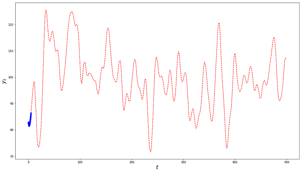Same draw as above but zoomed-out.

I’m sure you must be thinking that it looks more like what you’d expect from a stationary time series (e.g. it is visually mean-reverting). Let’s confirm that with our ADF test:

ADF Statistic: -4.2702p-Value: 0.0005Critical Values:	1%: -3.4440	5%: -2.8676	10%: -2.5700

Indeed, we can reject the null hypothesis that the time series is non-stationarity at a 0.05% p-Value, which gives us strong confidence.

However, the process hasn’t changed between the two experiments. In fact even the random path used is the same, and both experiments have enough points (at least a thousand each). So what’s wrong?

Intuitively, although the first experiment had a large enough sample size, it didn’t span long enough a time interval to be characteristic of the underlying process, and there is no way we could have known that beforehand!

The takeaway is that it is simply impossible to test whether a time series is stationary from a single path observed over a finite time interval, without making any additional assumption.

Two assumptions are often made but routinely overlooked by practitioners and researchers alike, to an extent that results in misinformed conclusions; an implicit assumption and an explicit assumption.

1. The Implicit Assumption

Stationarity is a property of a stochastic process, not of a path. Attempting to test stationarity from a single path ought to implicitly rely on the assumption that the path at hand is sufficiently informative about the nature of the underlying process. As we saw above, this might not be the case and, more importantly, one has no way of ruling out this hypothesis. Because a path does not look mean-reverting does not mean that the underlying process is not stationary. You might not have observed enough data to characterize the whole process.

Along this line, any financial time series, whether it passes the ADF test or not, can always be extended into a time series that passes the ADF test (hint: there exist stationary stochastic processes whose space of paths are universal). Because we do not know what the future holds, strictly speaking, saying that financial time series are non-stationary is slightly abusive, at least as much so as saying that financial time series are stationary.

In the absence of evidence of stationarity, a time series should not be assumed to be non-stationary — we simply can’t favor one property over the other statistically. This works similarly to any logical reasoning about a binary proposition A: no evidence that A holds is never evidence that A does not hold.

Assuming that financial markets are non-stationarity might make more practical sense as an axiom than assuming that markets are stationary for structural reasons. For instance, it wouldn’t be far fetch to expect productivity, global population, and global output, all of which are related to stock markets, to increase over time. However, would not make more statistical sense, and it is a working hypothesis that we simply cannot invalidate (in insolation) in light of data.

2. The Explicit Assumption

Every statistical test of stationarity relies on an assumption on the class of diffusions in which the underlying process’ diffusion must lie. Without this, we simply cannot construct the statistic to use for the test.

Commonly used (unit root) tests typically assume that the true diffusion is an Autoregressive or AR process, and test the absence of a unit root as a proxy for stationarity.

The implication is that such tests do not have as null hypothesis that the underlying process is non-stationary, but instead that the underlying process is a non-stationary AR process!

Hence, empirical evidence leading to reject the null hypothesis could point to either the fact that the underlying process is not an AR, or that it is not stationary, or both! Unit root tests by themselves are not enough to rule out the possibility that the underlying process might not be an AR process.

The same holds for other tests of stationarity that place different assumptions on the underlying diffusion. Without a model there is no statistical hypothesis test, and no statistical hypothesis test can validate the model assumption on which it is based.

Seek Stationary Alphas, Not Stationary Time Series

Given that we cannot test whether a time series is stationary without making an assumption on its diffusion, we are faced with two options:

• Make an assumption on the diffusion and test stationarity
• Learn a predictive model, with or without assuming stationarity

The former approach is the most commonly used in the econometrics literature because of the influence of the Box-Jenkins method, whereas the latter is more consistent with the machine learning spirit consisting of flexibly learning the data generating distribution from observations.

Modeling financial markets is hard, very hard, as markets are complex, almost chaotic systems with very low signal-to-noise ratios. Any attempt to properly characterize market dynamics — for instance by attempting to construct stationary transformations — as a requirement for constructing alphas, is brave, counterintuitive, and inefficient.

Alphas are functions of market features that can somewhat anticipate market moves in absolute or relative terms. To be trusted, an alpha should be expected to be preserved over time (i.e. be stationary in a loose sense). However, whether the underlying process itself is stationary or not (in the mathematical sense) is completely irrelevant. Value, size, momentum and carry are some examples of well documented trading ideas that worked for decades, and are unrelated to the stationarity of price or returns series.

But enough with stationarity, let’s move on to the nature of memory in markets.

Memory

Intuitively, a time series should be thought to have memory when its past values are related to its future values.

To illustrate a common misunderstanding about memory, let’s consider a simple but representative example. In Advances in Financial Machine Learning, the author argues that

“Most economic analyses follow one of two paradigms:

• Box-Jenkins: returns are stationary, however memory-less
• Engle-Ganger: Log-prices have memory, however they are non-stationary, and co-integration is the trick that make regression work on non-stationary time series […]”

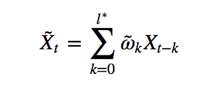
To get the best of both words, the author suggests constructing the weighted moving average process

whose coefficients are determined based on the notion of fractional differentiation with a fixed-window, as an alternative to log-returns (order 1 differentiation on log-prices). The author recommends choosing the smallest degree of fractional differentiation 0 < d < 1 for which the moving average time series passes the ADF stationarity test (at a given p-Value).

The whole approach begs a few questions:

• Is there really a dilemma between stationarity and memory?
• How can we quantify memory in time series so as to confirm whether or not they are memoryless?
• Assuming we could find a stationary moving average transformation with a lot of memory, how would that help us generate better alphas?

Quantifying Memory

Intuitively, it is easy to see that moving average processes exhibit memory by construction (consecutive observations of a moving average are bound to be related as they are computed in part using the same observations of the input time series). However, not every time series that has memory is a moving average. To determine whether stationary time series have memory, one ought to have a framework for quantifying memory in any time series. We’ve tackled this problem in our Yellow Paper, and here’s a brief summary.

The qualitative question guiding any approach to measuring memory in time series is the following. Does knowing the past inform us about the future? Said differently, does knowing all past values until now reduce our uncertainty about the next value of the time series?

A canonical measure of uncertainty in a random variable is its entropy, when it exists.

The entropy of a probability distribution with density function p with respect to a base measure dμ. The entropy of a random variable is that of its probability distribution.

Similarly, the uncertainty left in a random variable after observing another random variable is typically measured by the conditional entropy.

Conditional entropy of y given x.

A candidate measure of the memory in a time series is therefore the uncertainty reduction about a future value of the time series that can be achieved by observing all past values, in the limit case of an infinite number of such past values. We call this the measure of auto-predictability of a time series.

Measure of memory or auto-predictability of a time series.

When it exists, the measure of auto-predictability is always non-negative, and is zero if and only if all samples of the time series across time are mutually independent (i.e. the past is unrelated to the future, or the time series is memoryless).

In the case of stationary time series, PR({X}) always exists and is given by the difference between the entropy of any observation and the entropy rate of the time series.

Measure of auto-predictability of a stationary time series.

In our Yellow Paper, we propose a maximum-entropy based approach for estimating PR({X}). The following plot illustrates how much memory there is in stocks, futures and currencies.

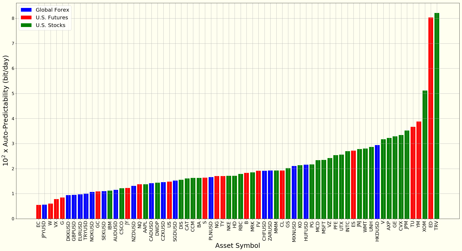Memory in daily returns of currencies, U.S. futures and U.S. stocks.

Memory Has Nothing To Do With Stationarity

A direct consequence of the discussion above is that a time series can both be stationary, and have a lot of memory. One does not preclude the other and, in fact, one is simply not related to the other.

Indeed, in the case of stationary Gaussian processes, it can be shown that the measure of auto-predictability reads

Measure of auto-predictability of a stationary Gaussian time series with power spectrum g.

It’s worth noting that PR({X})=0 if and only if the power spectrum is constant, that is, the time series is a stationary Gaussian white noise, otherwise PR({X})>0. A stationary white noise doesn’t lack memory because it is stationary, it lacks memory because it is, well […], a white noise!

The more uneven the power spectrum is, the more memory there is in the time series. The flatter the auto-covariance function, the steeper the power spectrum, and therefore the higher the measure of auto-predictability, and the more memory the time series has. An example such flat auto-covariance function is the Squared-Exponential covariance function

in the limit where the input length scale parameter l goes to infinity.

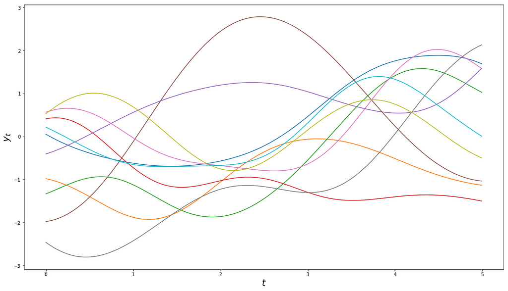Independent random draws from the same stochastic process, a mean-zero Gaussian process with Squared-Exponential covariance function, with output and input scale 1.

In short, there is no stationarity vs. memory dilemma. The confusion in practitioners’ minds comes from a misunderstanding of what goes on during iterated differentiation, as advocated by the Box-Jenkins methodology. More on that in the following section.

Memory Has Nothing To Do With Skewness/Kurtosis

Another misconception about memory (see for instance Chapter 5, page 83 of the aforementioned book) is that there is “skewness and excess kurtosis that comes with memory”. This is also incorrect. As previously discussed it is possible to generate time series that are Gaussian (hence neither skewed nor leptokurtic), stationary, and have arbitrarily long memories.

Iterated Differentiation, Stationarity And Memory

Iterated Differentiation Does Not Make A Time Series More Stationary, It Makes A Time Series More Memoryless!

Differentiation of (discrete-time) time series, in the Backshift Operator sense, works much like differentiation of curves learned in high-school.

The more we keep differentiating a curve, the more likely the curve will undergo a discontinuity/abrupt change (unless of course it is infinitely differentiable).

Intuitively, in the same vein, the more a time series is differentiated in the backshift operator sense, the more shocks (in a stochastic sense) the time series will undergo, and therefore the closer its samples will get to being mutually independent, but not necessarily identically distributed!

Once a time series has been differentiated enough times that it has become memoryless (i.e. it has mutually independent samples), it is essentially a random walk, although not necessarily a stationary one. We can always construct a non-stationary time series that, no matter how many times it is differentiated, will never become stationary. Here’s an example:

Example time series that cannot be made stationary by iterative differentiation. {W} is the standard Wiener process.

Its order-1 differentiation is completely memoryless as increments of the Wiener process are independent.

Its variance function g(t) is time-varying, and therefore {y} is non-stationary.

Similarly, the order-(d+1) differentiation of {y} is both memoryless and non-stationary for every d>0. Specifically, subsequent iterated differentiations read

and their time-dependent variance functions read

This expression clearly explodes in t for every d, and does not converge in d for any t. In other words, consecutive differentiations do not even-out the variance function, and therefore do not make this time series more stationary!

A Random Walk, Stationary Or Not, Would Typically Pass Most Unit-Root Tests!

The confusion in practitioners’ minds about iterated differentiation and stationarity stems from the fact that most unit root tests will conclude that a memoryless time series is stationary, although this is not necessarily the case.

Let’s consider the ADF test for instance.

Regression model underpinning the Augmented Dickey-Fuller test.

If a time series {y} is memoryless but not stationary, the Ordinary Least Square (OLS) fit underpinning the ADF test cannot result in a perfect fit. How would this departure be accounted for by OLS with a large enough sample? As the time series is memoryless, OLS will typically find evidence that γ is close to 1, so that the ADF test ought to reject the null hypothesis that γ=0, to conclude that the time series does not have a unit root (i.e. is a stationary AR). The time-varying variance of {y} will typically be observed by the stationary noise term {e}.

To illustrate this point, we generate 1000 random draws uniformly at random between 0 and 1, and we use these draws as standard deviations of 1000 independently generated mean-zero Gaussians. The result is plotted below.

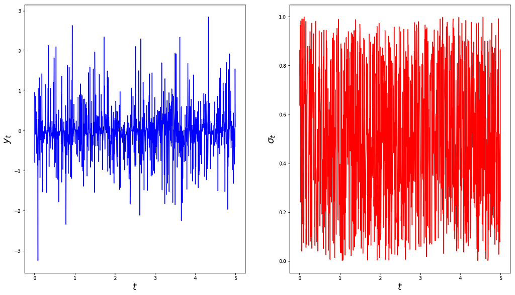A non-stationary memoryless time series (left) and its time-varying standard deviation (right).

An ADF test run on this sample clearly rejects the null hypothesis that the time series is a draw from an AR with unit root, as can be seen from the statistic below.

ADF Statistic: -34.0381p-Value: 0.0000Critical Values:	1%: -3.4369	5%: -2.8644	10%: -2.5683

At this point, practitioners often jump to the conclusion that the time series ought to be stationary, which is incorrect.

As previously discussed, a time series that is not a non-stationary AR is not necessarily stationary; it is either not an AR time series at all, or it is an AR that is stationary. In general the ADF test itself is inconclusive about which of the two assertions holds. In this example however, we know that the assumption that is incorrect is not non-stationarity, it is the AR assumption.

Concluding Thoughts

Much attention has been devoted to the impact AI can have on the investment management industry in the media, with articles riding the AI hype, warning about the risk of backtest overfitting, making the case that the signal-to-noise ratio in financial markets rules out an AI revolution, or even arguing that AI has been around in the industry for decades.

In these media coverages machine learning is often considered to be a static field, exogenous to the finance community, a set of general methods developed by others. However, the specificities of the asset management industry warrant the emergence of new machine learning methodologies, crafted with a finance-first mindset from the ground up, and questioning long-held dogmas. One of the biggest hurdles to the emergence of such techniques is perhaps the widespread misunderstanding of simple but fundamental notions, such as stationarity and memory, that are at the core of the research process.

Appendix: Code

Non-Stationarity and Memory In Financial Markets was originally published in Hacker Noon on Medium, where people are continuing the conversation by highlighting and responding to this story.