Simulating Portfolio Rebalances — When Does it Pay to Rebalance?

Simulating Portfolio Rebalances — When Does it Pay to Rebalance?

Imagine that your portfolio is comprised 50/50 of assets A and B. When the market shifts, the two assets not will always move in the same direction. Therefore, the portfolio will eventually drift away from its target allocation.

To maintain 50/50 composition, some of the better-performing assets must be sold in order to purchase the poorly performing asset. This is known as portfolio rebalancing. Portfolio rebalancing is used by investors to maintain their original asset allocations and risk level.

Sometimes, rebalancing can even be used to capture excess returns. It is a countercyclical strategy because it increases the allocation to the assets losing in value and decreases the allocation to the assets rising in value.

Put simply, rebalancing gives investors the opportunity to systematically “sell high and buy low”.

When a rebalanced portfolio outperforms an untouched, drifting portfolio, we call the excess return the “rebalancing bonus”.

Rebalancing Bonus = Annualized RoR for Rebalanced Portfolio — Annualized RoR for Drifting Portfolio

In this article, we’re going to demystify the rebalancing bonus phenomena and explore the circumstances under which it pays to rebalance.

Through simulations & analysis, I’m going to show that the rebalancing bonus is:

1. Decreased as the difference in long-term returns increases
2. Decreased further if this return difference is maintained over a long period of time
3. Increased by the volatility of each asset
4. Increased by a decreased correlation between each asset,
5. Maximized by an equal weighting of portfolio assets
6. Increased as the # of equally-weighted assets in a portfolio goes up
7. Not consistently affected by changes to the rebalancing frequency

Simulating Asset Returns via the Monte Carlo Method

For the sake of simplicity, we’re going to analyze the rebalancing bonus in a 50/50, two-asset portfolio.

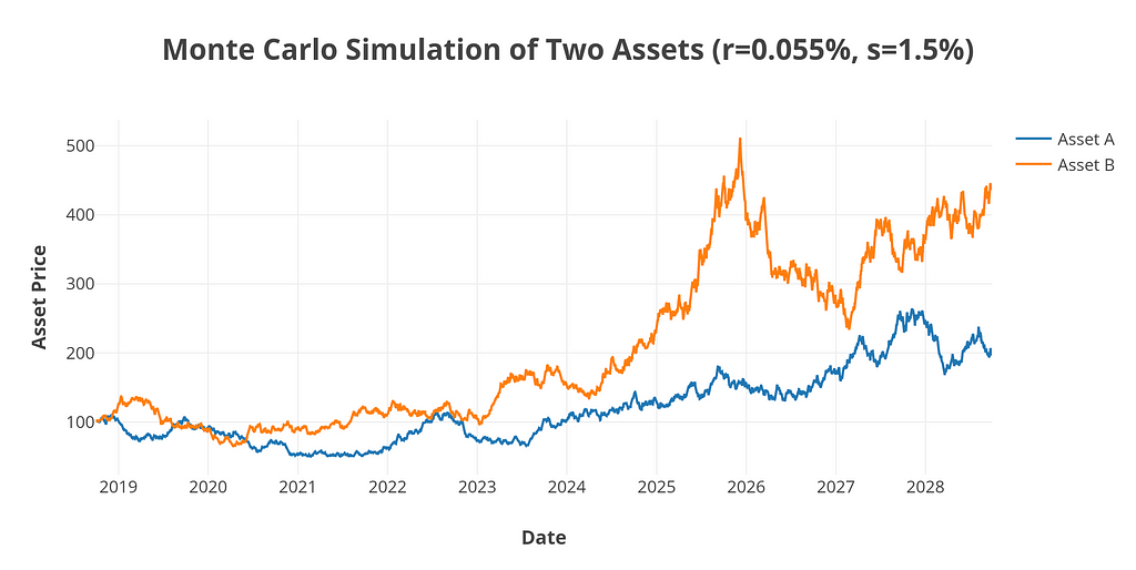
Our analysis will start by simulating prices-series data for a pair of assets over a 10-year period. These assets will have a defined mean and standard deviation. The price movements will follow Geometric Brownian Motion.

Here is an example of one simulation.

A Difference in Long-Term Returns Decreases the Rebalancing Bonus

A large return difference between the two assets in our portfolio means we are taking the returns from the higher performing asset, and re-allocating them into the lower performing asset every time we rebalance.

Let’s take a look at what the data yields after generating 1,000 simulations.

In the graph below, we plot the rebalancing bonus (%) on the Y-axis, and the absolute return difference between our two assets on the X-axis. Each dot on the plot represents a single simulation.

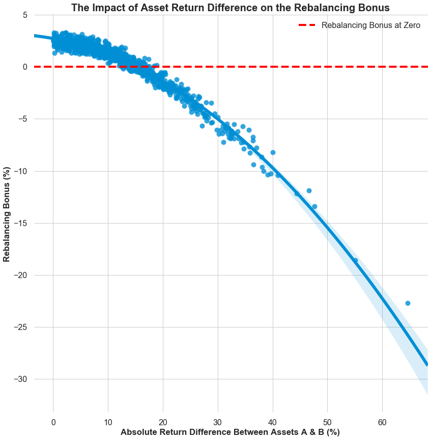1,000 simulations of a two asset portfolio over a 10 year period (r= 0.055%, s=1.5%, corr=0)

Simulations above the red line experience a positive rebalancing bonus, and dots below the red line suffer negative effects from rebalancing.

By following the non-linear, parabolic line of best fit, clearly, the rebalancing bonus only exists if returns between two assets are small enough. Otherwise, rebalancing will actually harm returns.

The Rebalancing Bonus Decreases if Return Differences Are Maintained Over Time

Because of the compounding effect, a slightly worse performing asset will continue to increasingly fall behind a better performing one. The longer return differences are maintained over time, the worse the rebalancing bonus will fare over time.

After simulating 500 portfolios across all 10, 25, and 50 year time periods, it’s clear that the rates of returns between two assets need to be smaller for longer investment horizons.

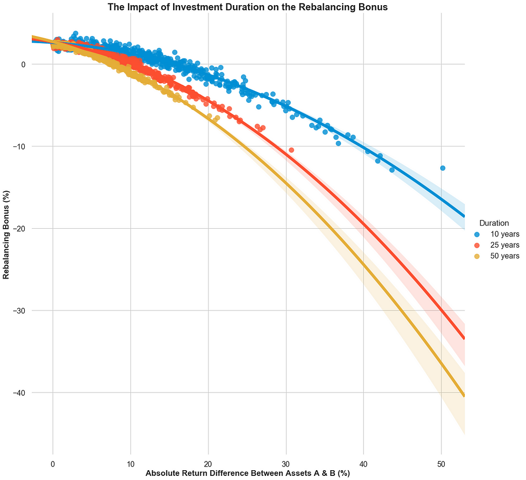500 simulations of a two-asset portfolio for each investment duration (r= 0.055%, s=1.5%, corr=0)Volatility Increases the Rebalancing Bonus

In the presence of high volatility, we will see asset prices oscillate back and forth. Intuitively, this should favour a rebalancing strategy by creating more opportunities to systematically “sell high and buy low”.

We’ll check this assumption by keeping mean and correlation constant while incrementing standard deviation by 0.01. We will run 500 simulations for each step.

As you can see, an increase in volatility increases the likelihood a rebalanced portfolio will outperform a drifting portfolio.

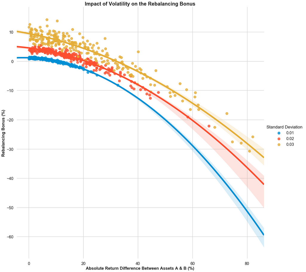1,000 simulations of a two asset portfolio over a 10 year period (r= 0.055%, corr=0)

As volatility increases, we are able to stomach a higher absolute difference in annualized returns between assets A & B.

However, with every unit of volatility added, it is also more likely that we will observe the different rate of returns between assets A and B. So while on average we may see a higher rebalancing bonus, our portfolio will become more and more susceptible to infrequent, but extreme differences in asset returns. Rebalancing when assets have extreme differences in return yields a negative bonus.

Positive Correlation Decreases the Rebalancing Bonus

Up to now, we’ve maintained a correlation coefficient of zero between each asset pair simulation. Each and every simulation is completely independent.

This is no longer the case. We’re going to use the Cholesky Decomposition to simulate correlated asset pairs.

To examine the impact of correlation, we’re going to keep our mean return and standard deviation constant. Instead, we’re going to use different correlation coefficients. We’ll run 500 simulations for each step.

From the data, we can see that as correlations increases between the asset pair, the rebalancing bonus decreases.

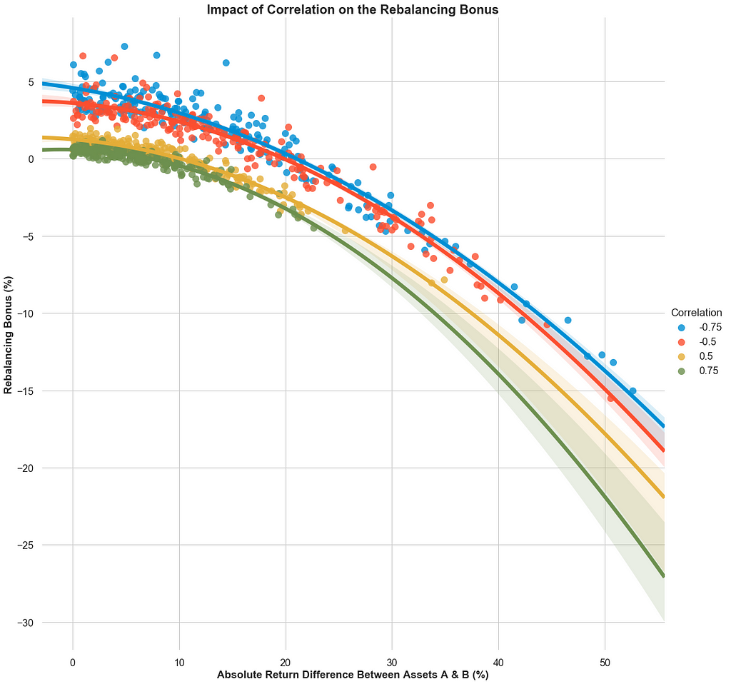1,000 simulations of a two asset portfolio over a 10 year period (r= 0.055%, s=1.5%)

When correlation increases, it reduces the return difference we can have between two assets and still yield a rebalancing bonus. As Bernstein succinctly stated, the intrinsic rebalancing potential of any asset pair is the difference between its mean-variance and covariance.

An Equally Weighted Portfolio Maximizes the Rebalancing Bonus

To examine the impact of different allocations in portfolio weights, we’re going to compare and contrast a 50/50 portfolio against one that one that is weighted 99/1.

Increasing the gap between weights should intuitively lower the rebalancing bonus. Our simulation confirms that it does.

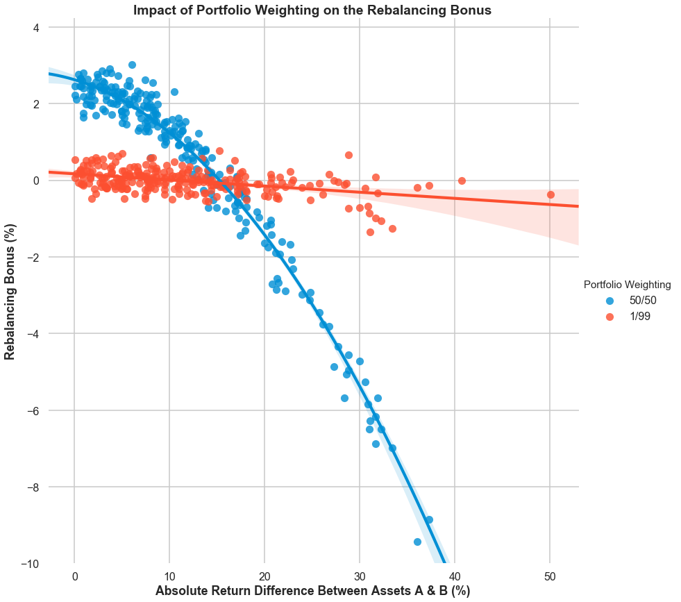1,000 simulations of a two asset portfolio over a 10 year period (r= 0.055%, s=1.5%, corr=0)

If the return difference between assets can be kept low, an equally-weighted allocation outperforms other portfolio weightings in maximizing the rebalancing bonus.

Increasing the # of Assets Improves the Rebalancing Bonus

As we increase the # of assets in our portfolio, the distance between the best-performing assets and the worst performing asset inevitably grows larger.

However as we increase the # of assets, portfolios are able to preserve a positive rebalancing bonus for larger, and larger return differences.

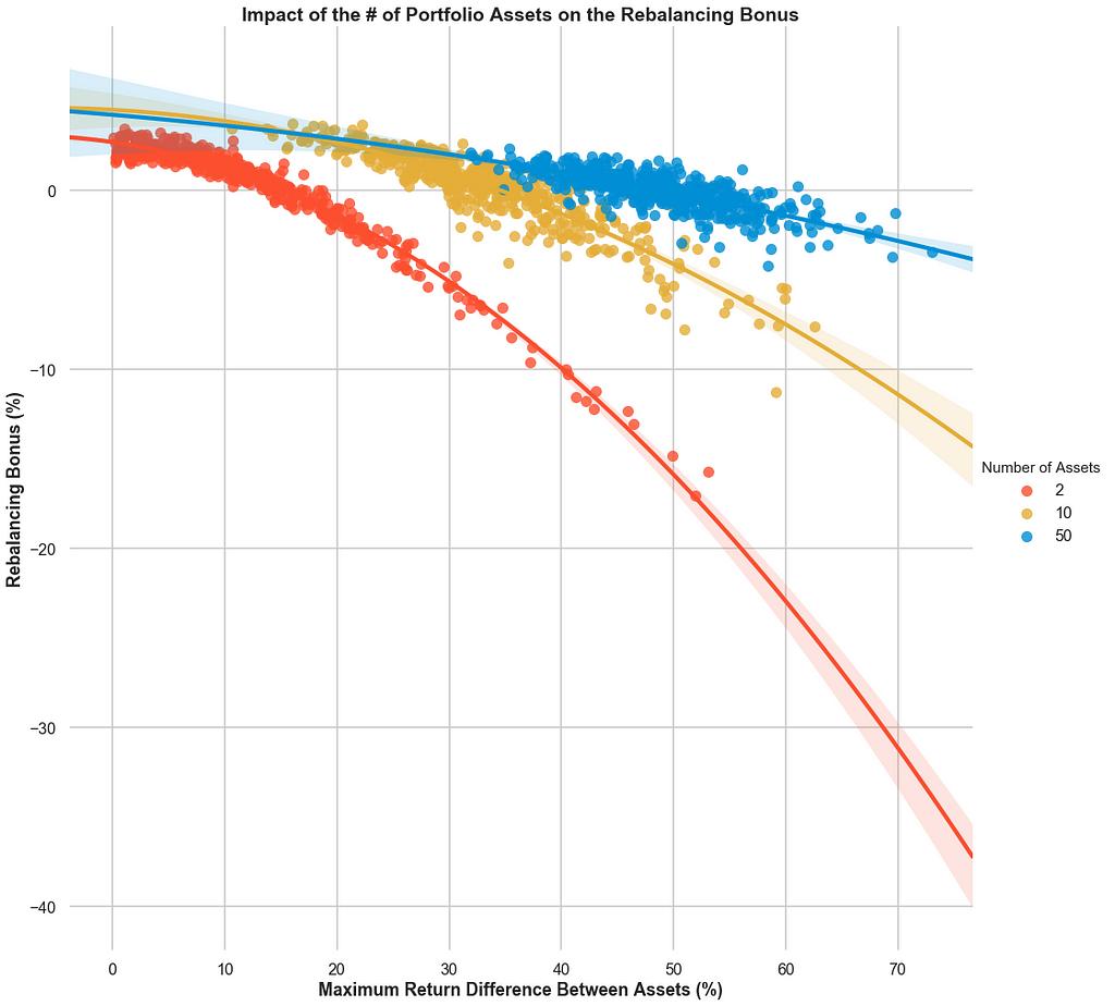500 simulations for each asset mix over a 10 year period (r= 0.055%, s=1.5%, corr=0)

Because these assets all have zero correlation, a larger and more diversified portfolio also reduces our risk.

The 50 asset portfolio captures a higher rebalancing bonus on average and has a higher minimum rebalancing bonus compared to the 2 asset portfolio.

How Much Does Rebalancing Frequency Matter?

Worst Case Scenario for Rebalancing

Given the worse case scenario for rebalancing:

• zero volatility
• large return difference between the assets
• large return difference that persists through time

There is no potential rebalancing bonus to be captured, therefore more frequent rebalancing is always worse, especially since it just incurs greater costs

There is no potential rebalancing bonus to be captured. The assets just drift further, and further away from one another.

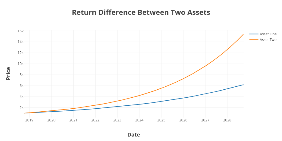Asset A has a r of 0.0055%. Asset B has a r of 0.0025%

In this scenario, more frequent rebalancing is always worse, especially once we factor in real-life trading costs.

Ideal Circumstance for Rebalancing

Given the best case scenario for rebalancing:

• negative correlations between two assets
• zero return difference between the two assets
• high volatility within each asset

In order to ensure a zero return difference between the two assets, we’re going to use a Brownian Bridge in our simulations. A Brownian Bridge follows Brownian motion but also ensures that the difference between the starting value, and end value is always zero.

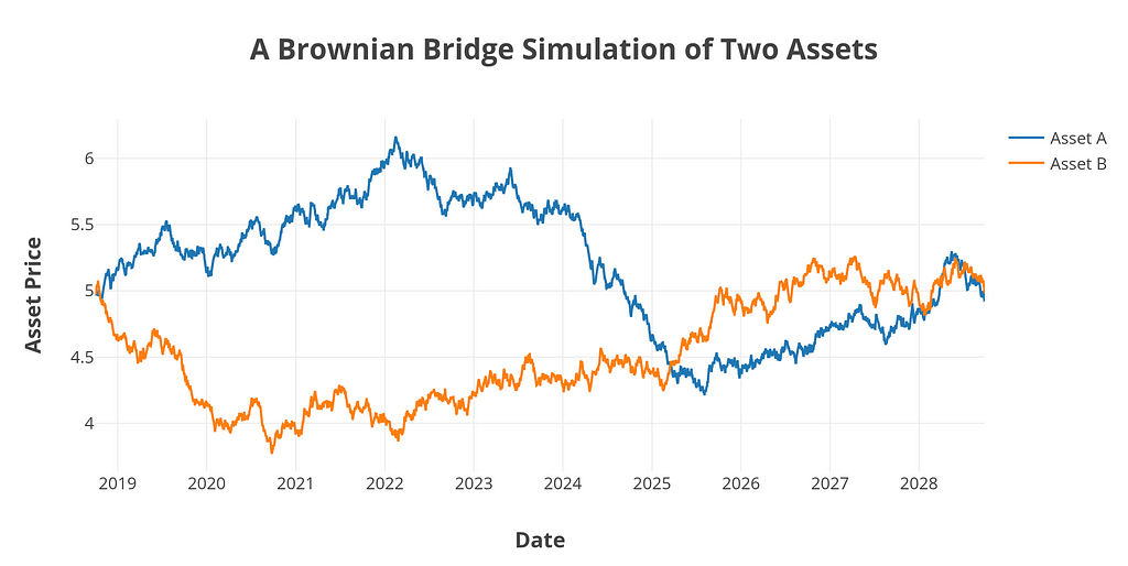Negatively Price starts at 5 and ends at 5, following a Geometric Brownian Motion

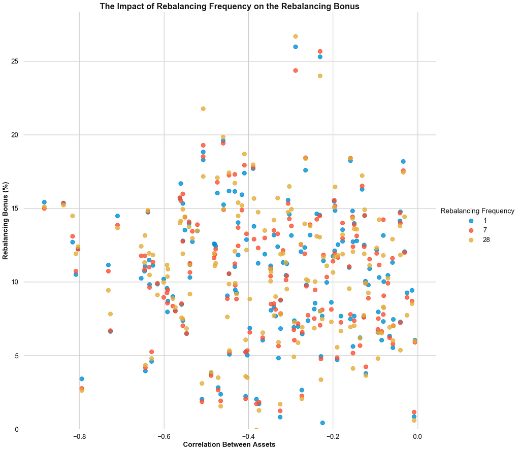
We’re going to use a different type of graph to show the result of the simulations. Since the return difference between assets is always zero, there’s no point plotting it on the X-axis. Instead, we’ll plot correlation on the X-axis, and keep rebalancing bonus on the Y-axis.

If more frequent rebalancing consistently improved the rebalancing bonus, the blue dots (1D) should consistently be plotted above the red (7D) and yellow dots (28D). We do not see that in our simulated data.

My guess is that rebalancing frequency only improves the rebalancing bonus if mean reversion happens at the same rate as the rebalancing frequency. Real world assets do not typically follow a consistent and predictable mean-reversion pattern, and neither do assets simulated via Geometric Brownian Motion.

For Cases that Fall in Between

The last check we’ll make is by simulating different rebalancing periods at different price volatilities.

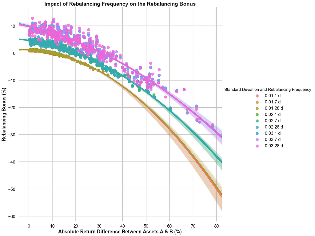500 simulations for each standard deviation over a 10 year period (r= 0.055%, s=1.5%, corr=0)

As we increase standard deviation, the non-linear half parabolic lines are clearly shifted up the Y-axis. However, changes in rebalancing frequency do not seem to have any consistent effect.

About the Author

I’m the founder of HodlBot.

We made a tool that automatically diversifies and rebalances your cryptocurrency portfolio. You can choose a long-term crypto index to DIY on your own exchange account. Or you can create your own custom portfolio.

I wrote this piece because a lot of HodlBot users had questions about portfolio rebalancing.

Join the Conversation

If you want to talk about this article, you should join our Telegram group of 300+ members.

HodlBot

Simulating Portfolio Rebalances — When Does it Pay to Rebalance? was originally published in Hacker Noon on Medium, where people are continuing the conversation by highlighting and responding to this story.