Latest news about Bitcoin and all cryptocurrencies. Your daily crypto news habit.
In this article, you get to look over my shoulder as I go about debugging a TensorFlow model. I did a lot of dumb things, so please don’t judge.
4. Rewrite from scratch in Keras
1 Goal of the ML model
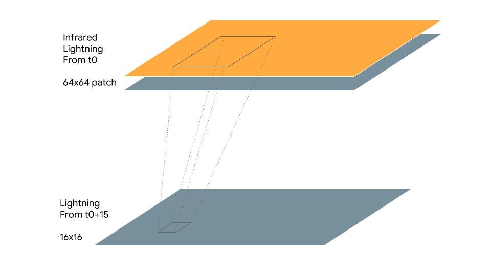
You can see the final (working) model on GitHub. I’m building a model to predict lightning 30 minutes into the future and plan to present it at the American Meteorological Society. The basic idea is to create 64x64 image patches around each pixel of infrared and Global Lightning Mapper (GLM) GOES-16 data and label the pixel as “has_ltg=1” if the lighting image actually occurs 30 minutes later within a 16x16 image patch around the pixel.
A model trained in this way can be used to predict lightning 30 minutes ahead in real-time given the current infrared and GLM data.
1a. Input function
I wrote up a convnet model borrowing liberally from the training loop of the ResNet model written for the TPU and adapted the input function (to read my data, not JPEG) and the model (a simple convolutional network, not ResNet).
The key bit of the code to get the input into a tensor:
parsed = tf.parse_single_example( example_data, {'ref': tf.VarLenFeature(tf.float32),'ltg': tf.VarLenFeature(tf.float32),'has_ltg': tf.FixedLenFeature([], tf.int64, 1), })parsed['ref'] = _sparse_to_dense(parsed['ref'], height * width)parsed['ltg'] = _sparse_to_dense(parsed['ltg'], height * width)label = tf.cast(tf.reshape(parsed['has_ltg'], shape=[]), dtype=tf.int32)Essentially, each TensorFlow record (created by an Apache Beam pipeline) consists of ref, ltg and has_ltg fields. The ref and ltg are variable length arrays that are reshaped into dense 64x64 matrices (using tf.sparse_tensor_to_dense). The label is simply 0 or 1.
Then, I take the two parsed images and stack them together:
stacked = tf.concat([parsed['ref'], parsed['ltg']], axis=1)img = tf.reshape(stacked, [height, width, n_channels])
At this point, I have a tensor that is [?, 64, 64, 2], i.e. a batch of 2-channel images. The rest of the input pipeline in make_input_fn (listing files, reading the files via parallel interleave, preprocessing the data, making the shape static, and prefetching) was essentially just copy-pasted from the ResNet code.
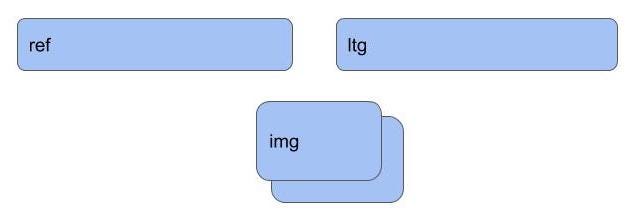 Stacking the two 4096-length arrays into a 3D tensor of shape (64, 64, 2)1b. Run the code
I developed the code by running the trainer locally for a few steps with a small batch size:
gcloud ml-engine local train \ --module-name=trainer.train_cnn --package-path=${PWD}/ltgpred/trainer \ -- \ --train_steps=10 --num_eval_records=512 --train_batch_size=16 \ --job-dir=$OUTDIR --train_data_path=${DATADIR}/train* --eval_data_path=${DATADIR}/eval*Then, I ran it on a larger dataset on Cloud ML Engine using a large machine with a heftier GPU:
gcloud ml-engine jobs submit training $JOBNAME \ --module-name=trainer.train_cnn --package-path=${PWD}/ltgpred/trainer --job-dir=$OUTDIR \ --region=${REGION} --scale-tier=CUSTOM --config=largemachine.yaml \ --python-version=3.5 --runtime-version=1.8 \ -- \ --train_data_path=${DATADIR}/train* --eval_data_path=${DATADIR}/eval* \ --train_steps=5000 --train_batch_size=256 \ --num_eval_records=128000 This was useful. Much of my debugging and development was done by running locally. This way I could work disconnected and didn’t need a GPU mounted on my machine.
2 Model doesn’t learn
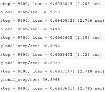
Once I had the code written and I ran it, I discovered that the model started quickly producing suspiciously identical losses:
and reached an accuracy metric that was stubbornly stuck at this number starting at epoch 1000:
'rmse': 0.49927762, 'accuracy': 0.6623125,
2a. The usual suspects
When a machine learning model won’t learn, there are a few usual suspects. I tried changing the initialization. By default, TensorFlow uses zeros_initializer. How about using Xavier (which uses small initial values), and setting the random seed for repeatability?
xavier = tf.contrib.layers.xavier_initializer(seed=13)c1 = tf.layers.conv2d( convout, filters=nfilters, kernel_size=ksize,kernel_initializer=xavier, strides=1, padding='same', activation=tf.nn.relu)
How about changing the gradient from the sophisticated AdamOptimizer to the trusty standby GradientDescentOptimizer?
How about reducing the learning rate from 0.01 to 1e-6?
None of these helped, but that’s what I first tried.
2b. Printing in TensorFlow
Was my input function perhaps returning the same data each time? That would explain why the model gets stuck. How do I know what the input function is reading in?
An easy way to verify that the input function is correct is to simply print out the values read. However, you can’t just print a tensor:
print(img)
That will simply print out the metadata of the tensor, not its values. Instead, you need to evaluate the value of the tensor while the program is being executed:
print(img.eval(sess=...))
and even that won’t work because the Estimator API doesn’t give you a handle to the session. The solution is to use tf.Print:
img = tf.Print(img, [img], "image values=")
What this does is to insert the print node between the original img node and the new img node, so that the value gets printed before the image node gets used again:
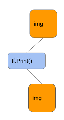 tf.Print() allows you to insert a printing node in the TensorFlow graph so that you can print out the values of a Tensor as the program executes.2c. Printing statistics of tensors
Once I did this, though, I got only the first 3 or 4 values (By default, tf.Print doesn’t print the whole tensor ) and they were mostly zero. Are they zero because satellite images tend to have a lot of zeros or is it zero because my input pipeline has a bug? Simply printing the image is not a great idea. So, I decided to print out statistics of the inputs:
numltg = tf.reduce_sum(labels)ref = tf.slice(img, [0, 0, 0, 0], [-1, -1, -1, 1])meanref = tf.reduce_mean(ref, [1, 2])ltg = tf.slice(img, [0, 0, 0, 1], [-1, -1, -1, 1])meanltg = tf.reduce_mean(ltg, [1, 2])
ylogits = tf.Print(ylogits, [numltg, meanref, meanltg, ylogits], "...")
The reduce_* functions in TensorFlow allow you to sum along an axis. Hence the first function reduce_sum(labels) computes the sum of the labels over the batch. Since the label is 0 or 1, this sum tells me the number of lighting examples in the batch.
I also want to print the mean of the reflectivity and lightning input image patches. For that, I want to do a sum over the height and width but keep each example and channel separate — that’s why you see [1,2] in the reduce_mean calls. The first tf.slice gets the first channel, and the second slice gets me the second channel (-1 in tf.slice tells TensorFlow to get all the elements in that dimension).
Notice also that I have inserted the Print node at the location of ylogits and get to print a whole list of tensors. This is important — you have to stick in the Print() into the graph at a node that actually gets used. If I had done:
numltg = tf.Print(numltg, [numltg, meanref, meanltg], "...")
the whole branch would have been optimized away since my model doesn’t actually use numltg anywhere!
Once I ran the code, I found that each batch had a good (and differing) mix of lightning points, that the means looked sort of similar within each batch, but were different from batch to batch.
2d. Fix the shuffle
Although this is not the problem we are trying to solve, this similarity of means by batch is quite odd. Looking over the code with this curiosity in mind, I found that I had hardcoded a shuffle size:
dataset = dataset.shuffle(1024)
Changing this to
dataset = dataset.shuffle(batch_size * 50)
resolved the batch problem.
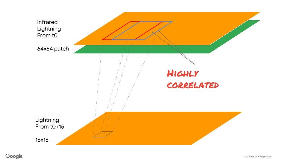 Because successive patches are highly correlated, it is important to shuffle in a large buffer
The issue is that because the data is created from sliding windows, successive examples tend to be highly correlated, so I need to shuffle over a large enough buffer that we get examples from a different part of the satellite image (or better still, different images). In the case of ResNet, each training example is a completely different image, so this is not an issue they were concerned about. Copy-paste strikes again!
2e. ReLu clips and saturates
But back to the original problem. Why are the accuracy and RMSE stuck? I kinda lucked out here. I had to insert the tf.Print() somewhere and so I stuck into a node that I knew I needed — on the output node of my model function (ylogits). I also happened to print out ylogits as well and lo and behold … while the inputs were all different values each time, ylogits started out random but quickly became zero.
Why is the ylogits zero? Looking carefully at the ylogits calculation, I noticed that I had written:
ylogits = tf.layers.dense( convout, 1, activation=tf.nn.relu, kernel_initializer=xavier)
Oops! By setting the ReLu activation function on the output dense layer, I had made sure ylogits would never be negative. Meanwhile, lightning is rarer than non-lightning, so the optimizer was pushing ylogits to the smallest possible value it could take. Which is zero. Because ReLu saturates below zero, it is possible for things to get stuck there.
The last-but-one-layer of a classification network is like the last layer of a regression network. It has to be:
ylogits = tf.layers.dense( convout, 1, activation=None, kernel_initializer=xavier)
Silly, silly, bug. Found and fixed. Whew!
3. NaN loss
Now, when I ran it though, I didn’t get a stuck accuracy metric. Worse. I got … “NaN loss during training.” If there is anything that will strike terror into the hearts of a ML practitioner, it’s NaN losses. Oh, well, if I can figure this thing out, I will get a blog post out of it.
As with a model that doesn’t train, there are a few usual suspects for NaN losses. Trying to compute cross entropy loss yourself is one of them. But I wasn’t doing that. I was computing the loss as:
loss = tf.reduce_mean( tf.nn.sigmoid_cross_entropy_with_logits( logits=tf.reshape(ylogits, [-1]), labels=tf.cast(labels, dtype=tf.float32)))
This should be numerically stable. The other problem is a learning rate that is too high. I switched back to AdamOptimizer and tried setting a low learning rate (1e-6). No go.
Another problem is that the input data might itself contain NaNs. This should not be possible — one of the benefits of using TFRecords is that the TFRecordWriter will not accept NaN values. Just to make sure, I went back to my input pipeline and added np.nan_to_num to the piece of code that inserted arrays into the TFRecord:
def _array_feature(value):value = np.nan_to_num(value.flatten())return tf.train.Feature(float_list=tf.train.FloatList(value=value))
Still no go.
3a. Simpler deep learning model
Maybe there are way too many weights? I made the number of layers in my model configurable and tried different numbers and smaller kernel sizes:
convout = imgfor layer in range(nlayers): nfilters = (nfil // (layer+1))nfilters = 1 if nfilters < 1 else nfilters# convolutionc1 = tf.layers.conv2d( convout, filters=nfilters, kernel_size=ksize, kernel_initializer=xavier, strides=1, padding='same', activation=tf.nn.relu)# maxpoolconvout = tf.layers.max_pooling2d(c1, pool_size=2, strides=2, padding='same')print('Shape of output of {}th layer = {} {}'.format( layer + 1, convout.shape, convout))outlen = convout.shape[1] * convout.shape[2] * convout.shape[3]p2flat = tf.reshape(convout, [-1, outlen]) # flattenedprint('Shape of flattened conv layers output = {}'.format(p2flat.shape))Still no go. The NaN loss remained.
3b. Back to linear
What if I completely remove the deep learning model? Remember my debugging statistics on the input image? What if we try to train a model to predict lighting based on just those engineered features:
halfsize = params['predsize']qtrsize = halfsize // 2ref_smbox = tf.slice(img, [0, qtrsize, qtrsize, 0], [-1, halfsize, halfsize, 1])ltg_smbox = tf.slice(img, [0, qtrsize, qtrsize, 1], [-1, halfsize, halfsize, 1])ref_bigbox = tf.slice(img, [0, 0, 0, 0], [-1, -1, -1, 1])ltg_bigbox = tf.slice(img, [0, 0, 0, 1], [-1, -1, -1, 1])engfeat = tf.concat([ tf.reduce_max(ref_bigbox, [1, 2]), # [?, 64, 64, 1] -> [?, 1]tf.reduce_max(ref_smbox, [1, 2]), tf.reduce_mean(ref_bigbox, [1, 2]), tf.reduce_mean(ref_smbox, [1, 2]), tf.reduce_mean(ltg_bigbox, [1, 2]), tf.reduce_mean(ltg_smbox, [1, 2])], axis=1)ylogits = tf.layers.dense( engfeat, 1, activation=None, kernel_initializer=xavier)
I decided to create two sets of statistics, one in a 64x64 box and the other in a 16x16 one and create a logistic regression model with just these 6 input features.
No go. Still NaN. This is very, very strange. A linear model should have never NaN-out. Mathematically, this is crazy.
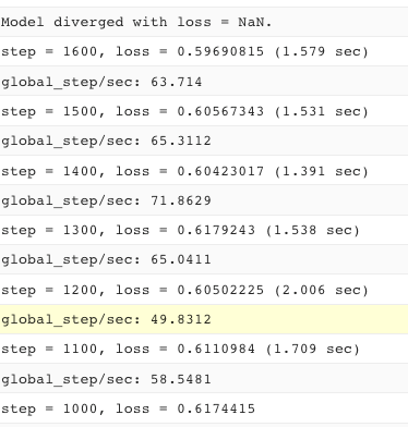
But just before it NaN-ed out, the model reached a 75% accuracy. That’s awfully promising. But this NaN thing is getting to be super annoying. The funny thing is that just before it “diverges” with loss = NaN, the model hasn’t been diverging at all, the loss has been going down:
Poking around to find out whether there is an alternate way to compute the loss, I discover that there is now a convenience function:
loss = tf.losses.sigmoid_cross_entropy(labels, tf.reshape(ylogits, [-1]))
Of course, that probably won’t fix anything but it’s better to use this function rather than call reduce_mean myself. But while here, let’s add asserts to narrow down the problem:
with tf.control_dependencies([ tf.Assert(tf.is_numeric_tensor(ylogits),[ylogits]), tf.assert_non_negative(labels, [labels]), tf.assert_less_equal(labels, 1, [labels])]): loss = tf.losses.sigmoid_cross_entropy(labels, tf.reshape(ylogits, [-1]))
Essentially, I assert that ylogits is numeric, and that each label is between 0 and 1. Only if these conditions are met do I compute the loss. Otherwise, the program is supposed to throw an error.
3d. Clip gradients
The assertions don’t trigger, but the program still ends with a NaN loss. At this point, it seems clear the problem does not lie in the input data (because I have done a nan_to_num there) or in our model calculation (because assertions don’t trigger) itself. Could it instead be in the back-propagation, possibly in the gradient computation?
For example, perhaps an unusual (but correct) example leads to unexpectedly high gradient magnitudes. Let’s just limit the effect of such unusual examples by clipping the gradient:
optimizer = tf.train.AdamOptimizer(learning_rate=0.001)optimizer = tf.contrib.estimator.clip_gradients_by_norm( optimizer, 5)train_op = optimizer.minimize(loss, tf.train.get_global_step())
That didn’t help either.
3e. L2 loss
If there are lot of very similar inputs, it is possible for the weights themselves to blow up. Over time, you might get a very high positive magnitude associated with one input node and a very high negative magnitude associated with the next input node. One way to get the network to avoid such a situation is to penalize high magnitude weights by adding an extra term to the loss function:
l2loss = tf.add_n( [tf.nn.l2_loss(v) for v in tf.trainable_variables()])loss = loss + 0.001 * l2loss
This gets all the trainable variables (weights and biases) and adds a penalty to the loss based on the value of those trainable variables. Ideally, we penalize just the weights (not the biases), but this is fine just for trying out.
3f. Adam epsilon
Poking around some more, I realize that the documentation for the AdamOptimizer explains the default epsilon value of 1e-8 may be problematic. Essentially, small values of epsilon cause instability even though the purpose of the epsilon is to prevent a divide-by-zero. This begs the question of why this is the default, but let’s try the larger value that is recommended.
optimizer = tf.train.AdamOptimizer( learning_rate=params['learning_rate'], epsilon=0.1)
That pushes the NaN further out, but it still fails.
3g. Different hardware
Another reason for this could be CUDA bugs and the like. Let’s try training on a different hardware (with P100 instead of Tesla K80) to see if the problem persists.
trainingInput: scaleTier: CUSTOM masterType: complex_model_m_p100
Still no go.
4. Rewrite as Keras
Sometimes, when left with an intractable bug, it is better to just try rewriting the model in a completely different way.
So, I decided to rewrite the model in Keras. This will also give me the opportunity to learn Keras, something I’ve been meaning to do for a while. Lemonade out of lemons and all that.
4a. CNN with Batchnorm
Creating a CNN with batchnorm (which will help keep gradients in range) is quite easy in Keras. (Thank you, Francois). So easy that I put batchnorm everywhere.
img = keras.Input(shape=[height, width, 2])cnn = keras.layers.BatchNormalization()(img)for layer in range(nlayers): nfilters = nfil * (layer + 1) cnn = keras.layers.Conv2D(nfilters, (ksize, ksize), padding='same')(cnn) cnn = keras.layers.Activation('elu')(cnn) cnn = keras.layers.BatchNormalization()(cnn) cnn = keras.layers.MaxPooling2D(pool_size=(2, 2))(cnn) cnn = keras.layers.Dropout(dprob)(cnn)cnn = keras.layers.Flatten()(cnn)ltgprob = keras.layers.Dense(10, activation='sigmoid')(cnn)Notice also that the final layer directly adds a sigmoid activation. There is no need to muck around with the logits because the optimization takes care of the numeric problems for us:
optimizer = tf.keras.optimizers.Adam(lr=params['learning_rate'])model.compile(optimizer=optimizer, loss='binary_crossentropy', metrics=['accuracy', 'mse'])
Nice!
Unfortunately (you know it by now), I still got NaNs!
Gaah. Okay, back to the drawing board. Let’s do all the things we did in TensorFlow in Keras.
4b. Feature engineering in Keras
First step is to forget about all this deep learning stuff and build a linear model. How do you do that? I have an image. I need to do feature engineering and send it to a Dense layer. That means, in Keras, that I have to write my own layer to do the feature engineering:
def create_feateng_model(params):# input is a 2-channel imageheight = width = 2 * params[’predsize’] img = keras.Input(shape=[height, width, 2]) engfeat = keras.layers.Lambda(lambda x: engineered_features(x, height//2))(img) ltgprob = keras.layers.Dense(1, activation=’sigmoid’)(engfeat)# create a modelmodel = keras.Model(img, ltgprob)
The engineered_features is exactly the same TensorFlow function as before! The key idea is that to wrap a TensorFlow function into a Keras layer, you can use a Lambda layer and invoke the TensorFlow function.
4c. Printing a layer
But I want to print out the layer to make sure that the numbers flowing through are correct. How do I do that? tf.Print() won’t work because, well, I don’t have tensors. I have Keras layers.
Well, tf.Print() is a TensorFlow function and so, use the same Lambda layer trick:
def print_layer(layer, message, first_n=3, summarize=1024):return keras.layers.Lambda((lambda x: tf.Print(x, [x], message=message, first_n=first_n, summarize=summarize)))(layer)
which can then be invoked as:
engfeat = print_layer(engfeat, "engfeat=")
4d. Clipping the gradient
Clipping the gradient in Keras? Easy! Every optimizer supports clipnorm.
optimizer = tf.keras.optimizers.Adam(lr=params['learning_rate'], clipnorm=1.)
Hey, I’m liking this Keras thing — it gives me a nice, simple API. Plus, it interoperates nicely with TensorFlow to give me low-level control whenever I need it.
 NaN is still there, slurping my milkshake
Oh, right. I still have the NaN problem
5. Unmasking the data
One final thing, something I kinda discounted. The NaN problem could also arise from unscaled data. But my reflectivity and lightning data are both in the range [0,1]. So, I don’t really need to scale things at all.
Still, I’m at a loose end. Why don’t I normalize the image data (subtract the mean, divide by the variance) and see if it helps.
 Yes, I’m clutching at straws now
To compute the variance, I need to walk through the entire dataset, and so this is a job for Beam. I could do this in TensorFlow Transform, but for now, let me hack it in Beam.
5a. Shuffling the training data in Beam
Since I am rewriting my pipeline, I might as well fix the shuffling issue (see section 2d) once and for all. Increasing the shuffle buffersize was a hack. I really don’t want to write the data in the order that I created the image patches. Let’s randomize the order of the image patches in Apache Beam:
# shuffle the examples so that each small batch doesn't contain# highly correlated recordsexamples = (examples | '{}_reshuffleA'.format(step) >> beam.Map(lambda t: (random.randint(1, 1000), t)) | '{}_reshuffleB'.format(step) >> beam.GroupByKey() | '{}_reshuffleC'.format(step) >> beam.FlatMap(lambda t: t[1]))Essentially, I assign a random key (between 1 and 1000) to each record, group by that random key, remove the key and write out the records. Now, successive image patches will not follow one after the other.
5b. Computing Variance in Apache Beam
How do I compute the variance in Apache Beam? I did what I always do, search on StackOverflow for something I can copy-paste. Unfortunately, all I found was an unanswered question. Oh, well, buckle down and write a custom Combiner:
import apache_beam as beamimport numpy as np
class MeanStddev(beam.CombineFn): def create_accumulator(self): return (0.0, 0.0, 0) # x, x^2, count
def add_input(self, sum_count, input): (sum, sumsq, count) = sum_count return sum + input, sumsq + input*input, count + 1
def merge_accumulators(self, accumulators): sums, sumsqs, counts = zip(*accumulators) return sum(sums), sum(sumsqs), sum(counts)
def extract_output(self, sum_count): (sum, sumsq, count) = sum_count if count: mean = sum / count variance = (sumsq / count) - mean*mean # -ve value could happen due to rounding stddev = np.sqrt(variance) if variance > 0 else 0 return { 'mean': mean, 'variance': variance, 'stddev': stddev, 'count': count } else: return { 'mean': float('NaN'), 'variance': float('NaN'), 'stddev': float('NaN'), 'count': 0 }[1.3, 3.0, 4.2] | beam.CombineGlobally(MeanStddev())Note the workflow here — I can quickly test it on a list of numbers to make sure it works.
Then, I went and added the answer to StackOverflow. Maybe all I need is some good karma …
5b. Write out mean, variance
I can then go to my pipeline code and add:
if step == 'train': _ = (examples | 'get_values' >> beam.FlatMap(lambda x : [(f, x[f]) for f in ['ref', 'ltg']]) | 'compute_stats' >> beam.CombinePerKey(MeanStddev()) | 'write_stats' >> beam.io.Write(beam.io.WriteToText( os.path.join(options['outdir'], 'stats'), num_shards=1)) )
Essentially, I pull out example[‘ref’] and example[‘ltg’] and create tuples that I group by key. Then, I can compute the mean and standard deviation of every pixel in both these images over the entire dataset.
Once I run the pipeline, I can print the resulting statistics:
gsutil cat gs://$BUCKET/lightning/preproc/stats*
('ltg', {'count': 1028242, 'variance': 0.0770683210620995, 'stddev': 0.2776118172234379, 'mean': 0.08414945119923131})('ref', {'count': 1028242, 'variance': masked, 'stddev': 0, 'mean': masked})Masked? What the @#$@#$@# does masked mean? Turns out that Masked arrays are a special numpy thing. Masked values are not NaN and so, if you process them with Numpy, nan_to_num() won’t do anything to it. On the other hand, it looks numeric, and so all my TensorFlow assertions don’t raise. Numeric operations with a masked value results in a masked value.
 Masked? What the @#@$#@ does masked mean?
Masked values are just like NaN — they will slurp your milkshake from across a room but the regular numpy and TensorFlow library methods know nothing about masking.
5c. Change masked values
Since the masking happens only in the reflectivity grids (I create the lightning grids myself by accumulating lightning flashes), I have to convert the masked values to a nice number after reading
ref = goesio.read_ir_data(ir_blob_path, griddef)ref = np.ma.filled(ref, 0) # mask -> 0
and now, when I rerun the pipeline, I get reasonable values:
('ref', {'count': 1028242, 'variance': 0.07368491739234752, 'stddev': 0.27144965903892293, 'mean': 0.3200035849321707})('ltg', {'count': 1028242, 'variance': 0.0770683210620995, 'stddev': 0.2776118172234379, 'mean': 0.08414945119923131})These are small numbers. There should be no reason to scale anything. So, let’s just train with the masking problem fixed.
This time, no NaN. Instead the program crashes and logs show:
Filling up shuffle buffer (this may take a while): 251889 of 1280000The replica master 0 ran out-of-memory and exited with a non-zero status of 9(SIGKILL)
5d. Reduce shuffle buffer size
Replica zero is the input pipeline (reading data happens on the CPU). Why does it want to read 1280000 records all at once into the shuffle buffer?
Well, now that the input data are so well shuffled by my Beam/Dataflow, I don’t even need that large a shuffle buffer (this used to be 5000, see Section 2d):
dataset = dataset.shuffle(batch_size * 50) # shuffle by a bit
And … 12 minutes later, the training finishes with an accuracy of 83%(!!!). No NaNs anywhere.
Woo hoo!
5e. Concatenate the models
Remember that we did only a linear model consisting of engineered features. Let’s add back the convnet in parallel. The idea is to concatenate the two dense layers, so that my model architecture can contain both the CNN layers and the feature engineering:
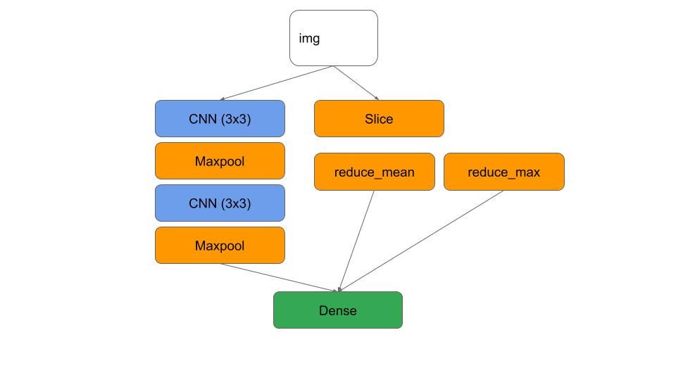 A combined model would be great
This is how to do this in Keras, with some batchnorm and dropouts thrown in, just because they are so easy to add:
cnn = keras.layers.BatchNormalization()(img)for layer in range(nlayers): nfilters = nfil * (layer + 1) cnn = keras.layers.Conv2D(nfilters, (ksize, ksize), padding='same')(cnn) cnn = keras.layers.Activation('elu')(cnn) cnn = keras.layers.BatchNormalization()(cnn) cnn = keras.layers.MaxPooling2D(pool_size=(2, 2))(cnn)cnn = keras.layers.Flatten()(cnn)cnn = keras.layers.Dropout(dprob)(cnn)cnn = keras.layers.Dense(10, activation='relu')(cnn)# feature engineering part of modelengfeat = keras.layers.Lambda(lambda x: engineered_features(x, height//2))(img)# concatenate the two partsboth = keras.layers.concatenate([cnn, engfeat])ltgprob = keras.layers.Dense(1, activation='sigmoid')(both)Now, I have an accuracy of 85%. This is still a small dataset (only 60 days of satellite data) and that’s probably why the deep learning path doesn’t add that much value. So, I’ll go back and generate more data, train longer, train on the TPU etc.
But those things can wait. Right now, I’m off to celebrate.
Debugging a Machine Learning model written in TensorFlow and Keras was originally published in Hacker Noon on Medium, where people are continuing the conversation by highlighting and responding to this story.
Disclaimer
The views and opinions expressed in this article are solely those of the authors and do not reflect the views of Bitcoin Insider. Every investment and trading move involves risk - this is especially true for cryptocurrencies given their volatility. We strongly advise our readers to conduct their own research when making a decision.
