Nearest Neighbors with Keras and CoreML

In this post, we will use Keras to build a cosine-based k-nearest neighbors model (k-NN) on top of an existing deep network. Finally (and optionally) we will convert the model to CoreML for use on iPhone or other iOS devices.

A Jupyter notebook with a complete code example is available here: https://github.com/sorenlind/keras-knn/

The basic problem is this: You have a set of images and you need to find images among them which are similar to a user image. Images, however, cannot easily be compared in their raw form, so you use a neural network to extract features (or representations, codes or encodings) from the images. These features can be compared using cosine similarity. So you want to build a cosine-based k-NN which for any given user image can find the k closest images in the database. It’s easy to build the k-NN using tools like Scikit-learn but for several reasons (detailed below), you want a single model that handles feature extraction and neighbor computation.

The solution is quite simple: Cosine similarity is basically just dot products (on normalized vectors). This means it can be easily expressed in Keras. In fact, it can be just a single dense layer with precomputed weights.

Why not Scikit?

Scikit-learn is a wonderful tool which lets you easily train and use many different Machine Learning models. And it lets you build k-NNs not only using cosine but with several other metrics as well. So, why not take advantage of that? There are several good reasons. Let’s see.

• Scikit-learn does not support GPUs. By building our k-NN in Keras, we can leverage GPUs for increased inference speed.
• Scikit-learn does not run on iOS devices. Apple’s tools for converting Machine Learning models to Apple’s CoreML format do support Scikit-learn but only some specific model types and the k-NN is not one of them. The Keras model, however, can be converted to CoreML, making it easy to run your model on an iPhone.
• Building the k-NN in Scikit-learn (or similar) would introduce another dependency. By building the k-NN with the same tools we use for the neural network, we can avoid introducing more dependencies.
• Having a single, unified model handling feature extraction and neighbor computation makes for a simpler setup.
• Finally, it’s a fun little exercise!

The Big Picture

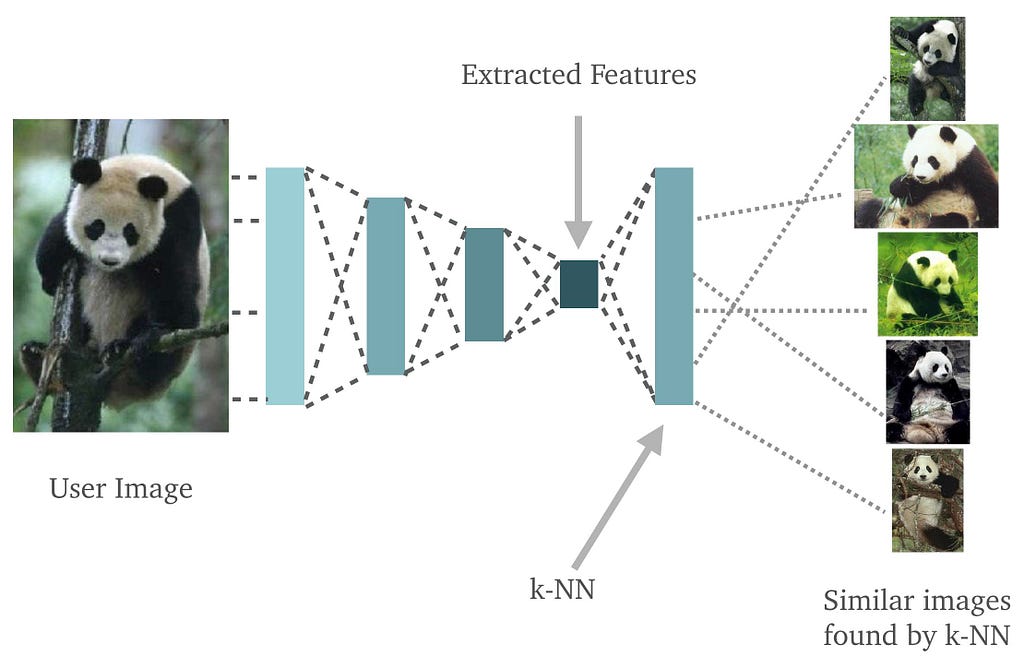
In broad terms, the flow of the system looks like this:

On the left we have the user image. We feed this through a convolutional network which extracts feature. The features are then fed through a dense layer which scores each image in the database by its similarity to the user image. Finally, we have the five most similar images as identified by the k-NN.

The steps we need to carry out are:

1. Obtain some images making up your image database.
2. Train or obtain a network for feature extraction.
3. Extract features for all images in the database.
4. Build a k-NN using the features extracted in step 3.
5. Join the feature extraction network and the k-NN for a single, unified model.

Let’s go through each step! And remember, for the complete code example, take a look at the Jupyter notebook.

Build the Image Database

Before we can do anything useful, we need some images. For this example, I will use images from the Caltech 101 dataset which contains images from 101 categories such as airplanes, butterflies, helicopters, pandas, pizzas and more. From the Caltech 101 website:

Pictures of objects belonging to 101 categories. About 40 to 800 images per category. Most categories have about 50 images. Collected in September 2003 by Fei-Fei Li, Marco Andreetto, and Marc ‘Aurelio Ranzato. The size of each image is roughly 300 x 200 pixels.

The Caltech101 dataset contains labeled images but we do not actually use the labels, so feel free to use an unlabeled dataset.

A Neural Network for Feature Extraction

To make things easy we will just use an off-the-shelf convolutional network trained for image classification, namely the ResNet50 network. We are not interested in the actual classification so we throw away the upper layers. This is really easy in Keras:

For real-world problems you could train your own network and use that instead. If you don’t have labeled data you could use a self-supervised approach such as autoencoders. But here, we will just stick with the ResNet50 network.

Extract Features

With our feature extraction network in place, we can now compute a feature vector for every image in our database. We call these our reference vectors. When a user sends us a new query image, we will extract a feature vector from the image (again using the feature extraction network). We call this the query vector. We will then compute cosine similarity between the query vector and each of the reference vectors and eventually pick the k images most similar to the query image. Normally, we would compute those cosine similarities using something like SciKit-learn but we will now see how it can be done in Keras using a dense layer.

How It Works

The math behind this little trick is actually really simple. To understand what is going on and how it works, we need to remind ourselves how the activation of a dense layer is computed and how the cosine is computed. This results in a few insights which are listed right below. We will go through each of them in more detail further down.

1. We can treat the reference vectors as column vectors and stack them horizontally to obtain a matrix which can be used as the weight matrix in a dense layer.
2. For the input vector x, the dense layer will compute the dot product x · w for every column vector w in the weight matrix W.
3. The cosine between two vectors x and w is defined as cos(x, w) = x · w / (|x|·|w|). Thus, the dense layer computes the cosine similarity multiplied by the product of the lengths of the two vectors.
4. A vector can be normalized, that is transformed to a vector of length 1 (a unit vector), without affecting the direction of the vector. Thus, normalizing a vector does not affect the cosine between that vector and any other vector. That is, if w’ is w normalized, cos(x, w) = cos(x, w’).
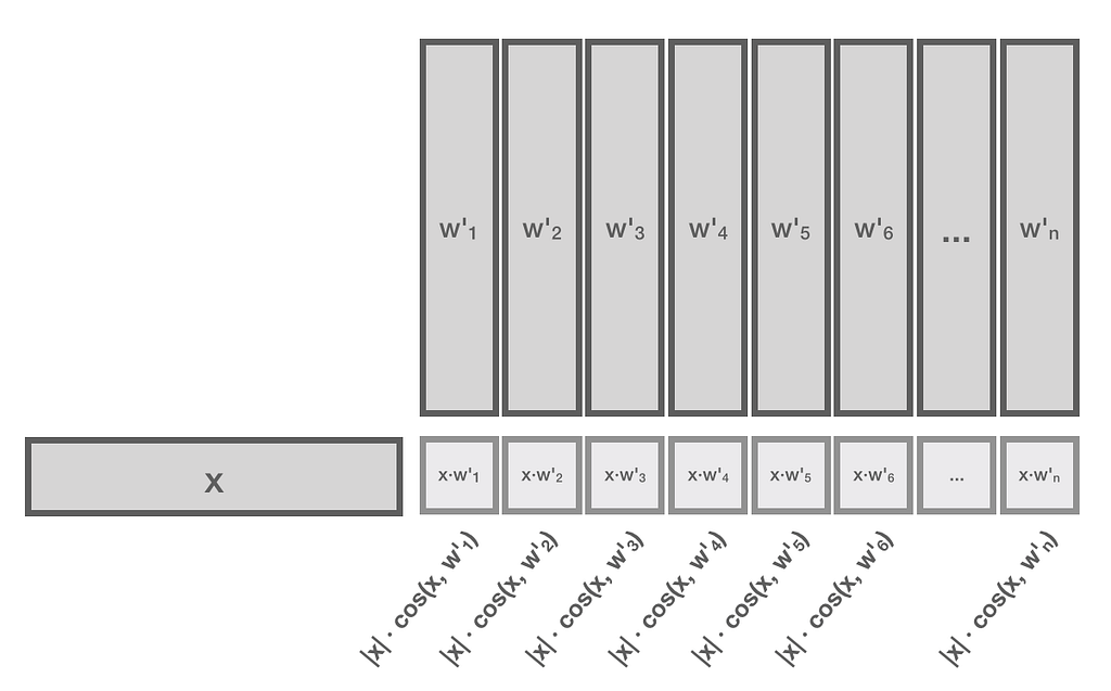
5. With w’ being a unit vector, its length is 1 and can consequently be removed from the cosine equation, resulting in cos(x, w’) = x · w’ / |x|. By multiplying by |x| on both sides we get that: x · w’ = |x|· cos(x, w’). Pairing that with insight number 2, we get that the dense layer will compute |x|· cos(x, w’) for the query vector x and every normalized reference vector w’ in the normalized weight matrix W’.
6. For any particular query vector x, the length |x| is constant. Therefore, for any particular query vector x, it holds that x · w’ ~ cos(x, w’), that is x · w’ is directly proportional to cos(x, w’). Consequently, to find the k most similar images, we can simplify the cosine computation to just x · w’.

Let us now look at each insight in a bit more detail!

1. Stacking Vectors

Having extracted a feature vector for each reference image, we can treat those reference vectors as column vectors and stack them horizontally to make up a matrix. This matrix can be used as the weight matrix of a dense layer in a neural network. This layer has the correct dimensions to take as input a feature vector (computed by the feature extraction network) and output a vector with dimensionality equal to the number of reference images. In our example, W will be of size 2048 by 9144. If you use another network or another dataset, you will, of course, see other dimensions.

2. Dense Layers Compute Dot Products

Let us now remind ourselves how the output or activation of a dense layer in a neural network is computed. With input vector x, weight matrix W, bias vector b and activation function g, the activation can be computed as:

a = g(x · W + b)

If we set the bias to 0 (by simply telling Keras to not use a bias) and use a linear activation we can simplify the activation as:

a = x · W

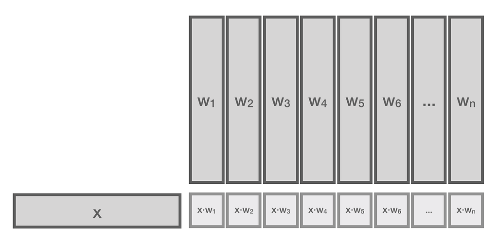
In other words, the activation of the dense layer (with no bias and a linear activation function) is simply the matrix product between the input vector x and the weight matrix W. Now, let’s remember that our W was made from stacking up reference vectors computed by feeding each image in our database through our feature extraction network. Thus, each element of the vector resulting from the matrix product x · W is actually the dot product between input vector x and a reference vector w. This can be illustrated as below:

As you can see, for each reference vector w, the dense layer computes x · w.

3. Cosine Similarity

As we briefly saw above, the cosine similarity between two vectors x and w is defined as cos(x, w) = x · w / (|x|·|w|). That is, the cosine similarity between two vectors is the dot product divided by the product of the lengths of the vectors. Now, we just saw in the previous section, that the dense layer basically computes a number of dot products, so this should be a hint that we could use the dense layer when computing the cosine similarities. We are not quite there yet, though. If we rewrite the cosine equation by multiplying by |x|·|w| on both sides (and flip the sides), we get the following:

x · w = |x|·|w|· cos(x, w)

Since x · w is exactly what the dense layer computes, we can now see that for the input vector x, a dense layer computes |x|·|w|· cos(x, w) for each column vector w in the weight matrix W.

4. Vector Normalization

We will now briefly change the focus and look for a moment at vector normalization. All we need to remember is that given two vectors, we can change the length of one or both of them without affecting the angle between them and consequently without affecting the cosine. This means we can transform all the vectors w in W to vectors w’ of length 1 (unit vectors) without affecting the cosine. We call this new matrix W’. In the next section we shall see how that makes computing the cosine simpler.

5. Simplifying the Cosine

We will now use the knowledge that our vectors, w’, are all of length 1 to simplify the cosine computation. As we saw above, the cosine definition can be rewritten as:

x · w’ = |x|·|w’|· cos(x, w’)

In contrast to before, we now know that one of the vectors, namely w’, is of length 1. This means multiplying by it has no effect, so we might as well remove it, which gives us:

x · w’ = |x|· cos(x, w’)

In other words, if we normalize all the reference vectors, the dense layer will compute |x|· cos(x, w’) for the query vector x and every normalized reference vector w’ in W’.

6. Proportionality

So, our dense layer computes |x|· cos(x, w’). But we set out to compute just cos(x,w’). We might consider simply dividing by |x|. Unfortunately, Keras has no division layer. TensorFlow has one, so we could use that. (This can be done in Keras with a Lambda layer in case you were wondering). But, if we take that approach, we will not be able to easily convert the model to CoreML (because the converter does not support Lambda layers unless you implement their computations in Swift/Objective-C and we do not want that). So we have to do something else, and luckily, the solution is simple: We can skip dividing by |x| entirely. For any given user image, dividing each of the dot products x · w’ by |x| has the effect of normalizing the cosine such that it’s a value between -1 and 1. But it’s the same operation applied to all the reference vector products (since|x| is constant for a given input image), and thus it does not change the ratio between them! Another way to put this is that for any particular query vector x, it holds that:

x · w’ ~ cos(x, w’)

That is x · w’ is directly proportional to cos(x, w’). Remember, we do not care about the actual cosine value. All we need is to find the k vectors in W’ which result in the greatest cosine. That is, we just need to be able to sort by the cosine values. Computing something that is proportional to the cosine for a particular query vector x suffices because this will result in the same order. In other words, computing x · w’ will suffice for our purpose — we are done!

For input vector x and every normalized vector w’ in W’, the dense layer computes |x|·cos(x, w’). Since |x| is constant for the particular input vector, it does not change the proportions.

That’s it for the math — we have seen that if we set the weights to the extracted reference feature vectors, the dense layer computes the dot products between the input feature vector and each of the reference vectors. And we have seen that these dot products are proportional to the cosine similarities if we just make sure to normalize the reference vectors. In short, all we have to do to find the k closest images is implement a dense layer with no bias and set its weights to the normalized feature weights!

There is one final and somewhat interesting note to make about our dense layer: As we have seen, the weights we use are computed by another network, namely the feature extraction network. This is unusual and therefore worth mentioning. Normally you would learn the weights using some variant of gradient descent and back-propagation but here they are computed in advance by another network!

Implementing with Keras

With the math out of the way, we can add the dense layer to the ResNet50 model:

Let’s now normalize the feature weights:

And finally set the weights of the network dense layer:

That’s all there really is to it! In the next section we will start making predictions using our new network.

Predictions

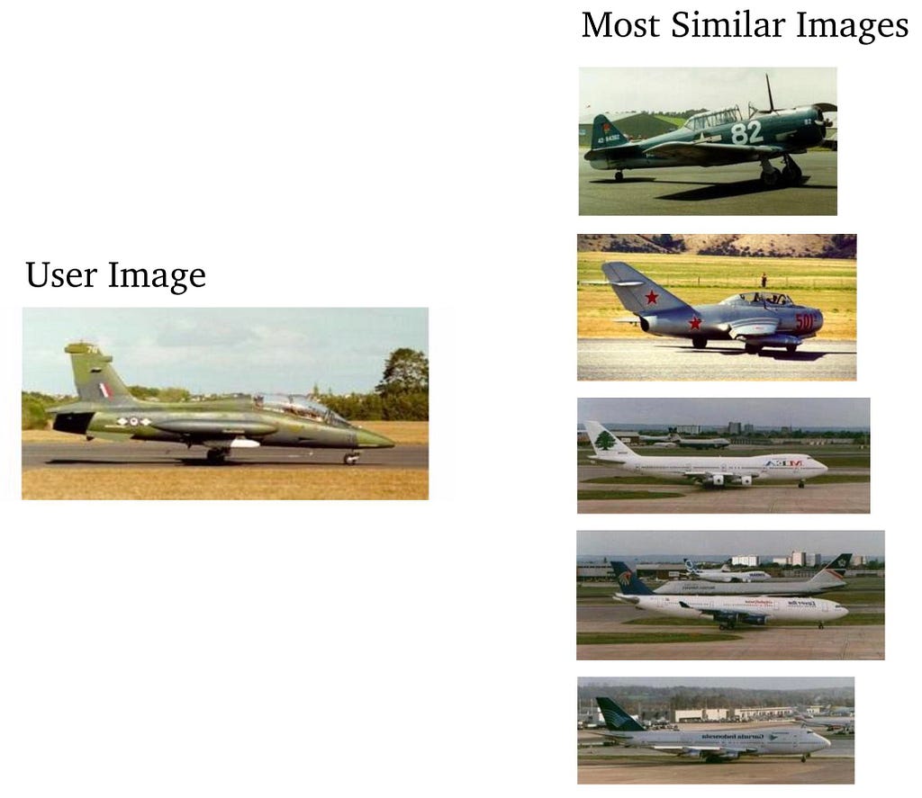
It is now time to make a few predictions using our network to see that it actually works!

Convert to CoreML

Having assured ourselves that the model works fairly well, we can now finally convert the model to CoreML as shown below.

A k-NN for Classification

You’ve now seen how to use the k-NN approach to search for similar images. Another (maybe even more interesting) application is to use it for image classification. This can be extremely useful because it can help you get away with using relatively few training examples even for problems with many thousand classes. If you think that sounds interesting, go and read my post on how I used an autoencoder and a k-NN to classify photos of over 35,000 different Magic cards!

Good luck and have fun implementing your own k-NN with Keras!

Nearest Neighbors with Keras and CoreML was originally published in Hacker Noon on Medium, where people are continuing the conversation by highlighting and responding to this story.