Key-point detection in flower images using deep learning

In this article we describe how we used a Convolutional Neural Network (CNN) to estimate the location of key-points in flower images. Key-points such as stem position and flower position are needed to render these images on a 3D model.

BloomyPro

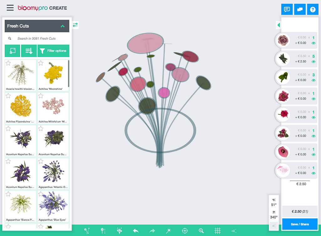
First, let’s introduce our client: Bloomy. Their software platform BloomyPro allows users to design their bouquets in the browser using a 3D model. It is used by breeders, retailers, wholesale and suppliers in the flower industry.

Instead of creating a real physical bouquet, taking a photo of it and sending it off to the client they can execute this process completely online. This saves them a lot of time and money.

The BloomyPro User Interface

To be able to compete with photos of real bouquets, the images created have to be as photo-realistic as possible. This is achieved by using real photographs of flowers from many angles and rendering them on a 3D model.

For every new flower they take photos from 7 different angles. In the photo booth, the flowers are automatically rotated by a motor.

The flower photo booth

In contrast, the post-processing of the pictures is not completely automated yet. There are currently thousands of flowers in the database and new flowers are added every day. Multiply this by the number of angles and you get a lot of pictures to process manually!

One of the post-processing steps is to locate a few key-points on the images needed for the 3D model to attach to. The most important ones are stem position and flower top position. This is now done manually. Our solution is aimed at automating this step.

Dataset

Fortunately thousands of images are already manually annotated with key-points. So we’ve got plenty of training data to work with!

Annotated images at different angles

Above are a few annotated flowers from the training set. It shows the same flower at a few different angles. The stem position is in blue and the flower top position in green.

In some pictures the stem origin is hidden by the flower itself. In this case we need an ‘educated guess’ where the stem is most likely to be.

Example with hidden stemNetwork architecture

Because the model has to output a number instead of a class we are essentially doing regression. CNN’s are best known for classification tasks but can also perform well on regression. For example DensePose does human pose estimation with a CNN based approach. Another example is this article about facial key-point detection.

I’m not going to explain the workings of convolutional networks in general, if you’re interested, you can read about CNN basics in this article:

A Beginner's Guide To Understanding Convolutional Neural Networks

The network begins with a few standard convolutional blocks. The blocks consist of 3 convolutional layers followed by a max-pooling, batch normalization and dropout layer.

• The convolutional layers contain a number of filters. Each filter works like a pattern recognizer. Next convolutional blocks have more filters so it can find patterns inside patterns.
• Max-pooling reduces the resolution of the image. This limits the amount of parameters in the model. Usually, with image classification, we’re not interested in where a certain object is located in the image, as long as it is there. In our case, we ARE interested in the location. Still, having a few max-pooling layers did not hurt performance.
• Batch normalization layers help the model to train (converge) faster. In some deep networks, training fails completely without them.
• Dropout randomly disables nodes and this prevents overfitting the model.

After the convolutional blocks we flatten the tensor so it becomes compatible with the dense layers. A global max-pooling or average max-pooling would also achieve a flat tensor but will lose all spatial information. Flattening worked better in our experiments, although it came at a (computational) cost of having more model parameters resulting in a longer training time.

After two dense hidden layers with Relu activation comes the output layer. We want to predict the x and y coordinates of the 2 key-points so we need to have 4 nodes in the output layer. The images can have different resolutions so we scale the coordinates to be between 0 and 1 and scale them back up before use.

The output layer has no activation function. Even though the target variables are between 0 and 1 this worked better for us than using a sigmoid.

For reference, here is the complete model summary from Keras, the Python deep learning library we used:

_________________________________________________________________Layer (type)                 Output Shape              Param #   =================================================================conv2d_1 (Conv2D)            (None, 126, 126, 64)      2368      _________________________________________________________________conv2d_2 (Conv2D)            (None, 124, 124, 64)      36928     _________________________________________________________________conv2d_3 (Conv2D)            (None, 122, 122, 64)      36928     _________________________________________________________________max_pooling2d_1 (MaxPooling2 (None, 61, 61, 64)        0         _________________________________________________________________batch_normalization_1 (Batch (None, 61, 61, 64)        256       _________________________________________________________________dropout_1 (Dropout)          (None, 61, 61, 64)        0         _________________________________________________________________conv2d_4 (Conv2D)            (None, 59, 59, 128)       73856     _________________________________________________________________conv2d_5 (Conv2D)            (None, 57, 57, 128)       147584    _________________________________________________________________conv2d_6 (Conv2D)            (None, 55, 55, 128)       147584    _________________________________________________________________max_pooling2d_2 (MaxPooling2 (None, 27, 27, 128)       0         _________________________________________________________________batch_normalization_2 (Batch (None, 27, 27, 128)       512       _________________________________________________________________dropout_2 (Dropout)          (None, 27, 27, 128)       0         _________________________________________________________________flatten_1 (Flatten)          (None, 93312)             0         _________________________________________________________________dense_1 (Dense)              (None, 256)               23888128  _________________________________________________________________batch_normalization_3 (Batch (None, 256)               1024      _________________________________________________________________dropout_3 (Dropout)          (None, 256)               0         _________________________________________________________________dense_2 (Dense)              (None, 256)               65792     _________________________________________________________________batch_normalization_4 (Batch (None, 256)               1024      _________________________________________________________________dropout_4 (Dropout)          (None, 256)               0         _________________________________________________________________dense_3 (Dense)              (None, 4)                 1028      =================================================================Total params: 24,403,012Trainable params: 24,401,604Non-trainable params: 1,408_________________________________________________________________

You might ask: why 3 convolutional layers? Or why 2 convolutional blocks?We included these numbers as hyperparameters in a hyperparameter search. Together with parameters such as: number of dense layers, dropout level, batch normalization and the number of convolutional filters we did a randomized search to find the optimal combination of hyperparameters.

And why randomized search instead of grid search? It’s a little counter intuitive but in practice this gives you better results for your money. See also this article about hyperparameter tuning.

For training we use the Adam optimizer with a learning rate of 0.005. The learning rate is automatically reduced when the validation loss is not improving for a few epochs.

As loss function we use Mean Square Error (MSE). Thus, large errors are punished relatively more than small errors.

Training and performance

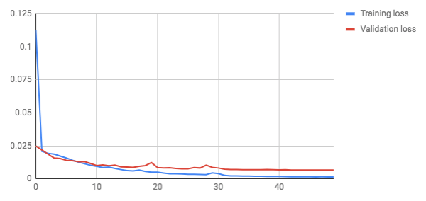
These are the loss (error) plots after training for 50 epochs:

Loss plots

After about 8 epochs, the validation loss becomes higher than the training loss. The validation loss still decreases up to the end of training so we see no signs of the model strongly overfitting.

The final loss (MSE) on the test set was 0.0064. MSE can be quite unintuitive to interpret. Mean Average Error (MAE) is a bit easier to explain to humans.

The MAE is 0.0017— This means that the predictions are on average 1.7% off

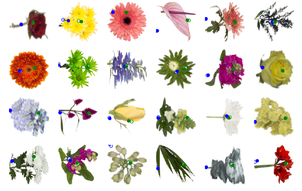
See below for a few examples of the test set. The white circles contain the target key-points and the filled circles our prediction. They are pretty close (overlapping) in most cases.

Some images from the test setDeployment

The performance of the model is good enough to add value to the product. The key-points are now used to set default coordinates when uploading new flower images. In most cases no manual adjustment is needed!

The model itself is exposed via an API and packaged in a docker container. This container is built on push via bitbucket pipelines. The trained weights are also contained in the docker image. As you don’t want large files in Git we use Git LFS to store them.

Further improvements

We got some idea’s for improvement that we didn’t have time for yet to implement:

1. Currently a single model is estimating both key-points. It might work better to train a specific model per key-point. This has the additional benefit that you can add new key-points later without having to retrain the complete model.
2. Another idea is to take the angle of the photograph into account. For example by adding it as input of the dense layers. You could argue that the angle changes the nature of the task so providing this information might help the network. In this line of thought training a separate network for each angle could also be beneficial.

Next steps