Link Prediction In Large-Scale Networks

A comparison of supervised and unsupervised approaches to infer missing links from an observed network.

by Guillaume Le Floch (Data Scientist at Cdiscount)

What is the point of predicting new links when you already have plenty of them ?

If you have decided to read this article, you must either be very interested in Data Science or extremely bored right now. Whether this is the first or the second option, we are delighted to have you on board and wish that you will enjoy the ride through the link prediction problem with us.

On a more serious note, the goal of this paper is to find the best option to predict accurately future connections in a graph, which you can also call a network. Not a tiny, harmless network. No, we are talking about large-scale networks. The big and horrendous ones made of billion of nodes and edges which Facebook, Google (and Cdiscount) have had to deal with on a daily basis for the last few years.

What is the point of predicting new links when you already have plenty of them ?

We have seen this question coming from a mile away, and we have got you covered, don’t worry. It is in the human nature (and even more in the Data Scientist one), to want more than what we already have. We don’t settle for the present, we want to know the future as well. Therefore, we need to find a way to perform predictions as accurate as possible.

Furthermore, a network is what we can call a dynamic structure as it evolves with time. For instance, social networks such as Facebook, Twitter, LinkedIn etc. change permanently as new connections appear while some others are removed from the graph.

For this particular example, one of the biggest challenges is to make accurate recommendations to the users. They may know somebody in real life, but aren’t connected with that person on their favourite social network. Thus, the target in this case would be to predict (and recommend) this association (link in the graph), in order to fix what can be seen as a mistake.

Link prediction can help rebuild the real life, but it could actually do more than just that. What we observe isn’t always ideal. An example would be terror attacks : given relationships between terrorists, you can build a network which represents who worked with who in the past. Link prediction can help predict future associations, allowing a government to monitor suspects and prevent them from committing a terror attack together. Biology is another area where link prediction can be a key asset, as human brains aren’t enough to predict all associations between molecules, having an artificial intelligence to do the job can be a massive boost.

To put it in a nutshell, link prediction can be used for various purposes, in many different areas. In this article, we will focus mainly on the collaboration network case. We will work with the DBLP dataset (See [1] for more details). This is a co-authorship network where two authors are connected if they publish at least one paper together, so we will try to predict relevant future collaborations here (we would like to avoid awkward situations).

The learning context: unsupervised vs. supervised

In this section, we will discuss the possibilities at our disposal to perform predictions in a graph. As this is a special structure, we need to clarify a few points before getting started with prediction. Let’s start with a bit of theory and notations before practising.

A little reminder of Graph Theory

To ensure we are all speaking about the same things, let’s use the same vocabulary about graphs. And even if you already know this, a little reminder does no harm:

From a mathematical point of view, a graph can be defined as G = (V, E) with V being the set of nodes (or vertices) and E the set of edges.
A graph is undirected if the relationship goes both ways. Facebook is a good example of that : when someone is your friend, you automatically are his friend too. On the contrary, a graph is directed if the link goes from one node to another, but it isn’t reciprocal. Twitter illustrates this perfectly as you can follow somebody, but this individual doesn’t necessarily follow you in return.
We can define the graph’s adjacency matrix (of dimension |V| × |V|) as A = [A_ij] with (i, j) ∈ V. For an undirected and unweighted graph :

A sequence is a succession of consecutive edges : {i_1, i_2}, {i_2, i_3}, …, {i_K-1, i_K}.
A path between nodes i and j is a sequence of edges {i_1, i_2}, {i_2, i_3}, …, {i_K-1, i_K} such as i_1 = i and i_K= j and each node in the sequence is distinct.
As we are going to heavily use the concept of neighborhood, let’s denote 𝛤(u) the set of nodes which are directly linked with the node u (they are its “neighbors”).
A distance between two nodes is given as the minimal number of edges to go from one node to another (shortest path).

The DBLP dataset which will be used for our experiments has the following properties:

317,080 nodes (researchers).
1,049,866 edges (co-autorships between researchers).

Yes, you are right. This is what we can call a large-scale network, and this is ideal in order to perform learning tasks, whether they are supervised or unsupervised. This will provide us with stability and confidence in the results we will get from the experiment.

Let’s now discover the learning process in the next part(s).

The Creation of Training, Test and Validation Sets

The part we are entering is a tricky one, so fasten your seat belt, we don’t want to lose you now. Splitting a dataset into training/test/validation sets isn’t a difficult concept to understand in normal circumstances. When it comes to graphs, it is a bit different. How can you split a graph to achieve a learning task ? First of all it is important to remember precisely our purpose : we want to predict links (edges) between nodes.

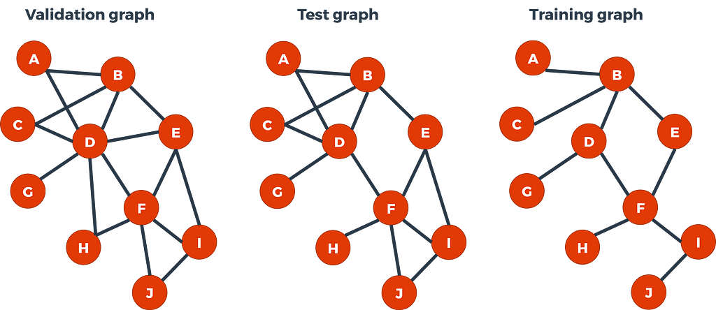
The first capital information is the following one : the predictive algorithm will take as input node pairs and evaluate whether the nodes present the properties to be linked in the future. In this paper, we will only look at nodes which are at distance 2. What remains to be clarified now is the output : how can we create ground-truth labels from the graph ? The idea is to take a graph, hide some of its edges and monitor the results produced by the algorithm. For hidden links the label is 1, for non-existent links it is 0. Not clear enough yet ? No problem, let’s illustrate the concept with a minimal example :

From the left to the right we have :

The “validation graph” which denotes as G_valid = (V, E_valid) with : V = {A, B, C, D, E, F, G, H, I, J} and E_valid = {(A,B); (A, D); (B, C); (B, D); (B, E); (C, D); (D, E); (D, F); (D, H); (D, G); (E, F); (E, I); (F, H); (F, I); (F, J); (I, J)}.
The “test graph” where we have hidden two edges : G_test = (V, E_test) with E_test = E_valid \ {(D, E); (D, H)} thus E_test ⊂ E_valid.
The “training graph” where we have hidden four more edges : G_train = (V, E_train) with E_train = E_test \ {(A, D); (C, D); (E, I); (F, J)} thus E_train ⊂ E_test.

So, as you can see it is not that deep, it is just a matter of a graph which contains a subgraph which itself contains a subgraph…

If you are still firmly with us at this point, then you have understood that our training set (with the corresponding labels) looks like the table below.

Make no mistake, the edge (D, H) for example has the label 0 here because it doesn’t exist in the Test Graph, even though it was originally present in the Validation Graph.

As we are evaluating all the 2-hop “missing link” node pairs we can see that the edges we have hidden have label of 1 while the rest have a label of 0. Let’s remember that this is just a minimal example, although we can already see several interesting facts :

The number of node pairs to evaluate is fast-growing, we will let you imagine how it is like in a large-scale network (we will see it afterwards anyway).
The problem of class imbalance appears : there are far more 0 labels, so we will have to deal with this problem later on..

Let’s now discover what are the unsupervised methods we can choose to perform link prediction in a graph, digging deepeer into the notions of neighborhood and local similarity in the process.

Unsupervised Learning : The Notion of Similarity Indices and Neighborhood

If the nodes in the graph don’t possess properties, as is the case in our study, the only information available comes from the topological structure of the graph. By that, we mean the neighborhood of a node : how many neighbors has this node got ? How many neighbors these neighbors themselves have ? How are they organised ? As we are evaluating node pairs we can also look at how similar a node u can be to a node v by looking at their “distance” in the graph, the similarity of their local neighborhood.

All of this has led to several local similarity indices such as Common Neighbors, Jaccard Similarity, Adamic-Adar Index, Resource Allocation, etc (more can be found in [2] and [3]). These indices will return a score s ∈ ℝ which will be used to perform predictions. As it is explained in [3], you will also need to set a threshold value above which you assign the label 1. We sense that you may be asking which unsupervised method is the best to perform predictions. This is a tricky question as in some cases, one measure will outperform others, but in other cases it will be another one, etc.

And what if we didn’t actually have to choose ? What if we let something else combine those local similarity indices to get a score in return ? You’ve got it right, we are heading straight to the Supervised Learning universe.

Feature Engineering for Supervised Learning

We have already discussed how to obtain labels. Now we need features in order to perform Supervised Learning (Binary Classification). And yes, you guessed it, these features will come from the latest part we discussed. Based on Kolja Esders’s work in [3], we will use unsupervised scores as features for our predictive model. We will also use the notion of Community (further details can be found in [4]).

The following features will be included in our learning/prediction task : Common Neighbors (CN), Jaccard Coefficient (JC), Adamic-Adar index (AA), Resource Allocation (RA), Preferential Attachement (PA), Adjusted-Rand (AR) and Neighborhood Distance (ND) which are all local indices to which we will add the Total Neighbors (TN), Node Degree (UD et VD) and Same Community (SC) features. They are defined as:

As for Adjusted-Rand here is a table giving the meaning of a, b, c and d :

Before going into predictions, we just need to discuss the evaluation metric which will help us determine whether Supervised Learning is better than the Unsupervised one (Spoiler alert : from Kolja Esders and our own experience in the past, it seems that it is the case) and it happens in the very next part.

Evaluation metric

The evaluation metric chosen in this study is a well-known one : the AUC. As it is a binary classification problem, it is ideal and will also allow us to plot the ROC curves of the method to illustrate the comparison between algorithm results. This will also free us from having to set a threshold for the unsupervised method.

Considering two independent and identically distributed observations (X1; Y1) and (X2; Y2), the AUC of a scoring method S can be written in the following manner :

In other words, a perfect algorithm (which would get an AUC of 1) would give higher scores to every node pairs having a label of 1 than node pairs having a label of 0. This is just a matter of score order, whichever score is used.

In the next section we will put several algorithms face to face in the arena and compare their performances :

Resource Allocation (Unsupervised Method)
Adamic-Adar (Unsupervised Method)
Jaccard Coefficient (Unsupervised Method)
Common Neighbors (Unsupervised Method)
Tree-based XGBoost (Supervised Method, combination of unsupervised scores with other features)

Experiments on the DBLP Dataset

Before plotting the ROC curves and unleash the results, we will talk about data processing. As we pointed out previously, the class imbalance problem appears when dealing with huge networks. So after finding all the 2-hop missing links in our training and test graphs, we decided to randomly drop samples with labels zero in order to get a 50/50 balance for labels. This has led to these datasets :

Train : 277,742 samples (node pairs).
Test : 150,348 samples (node pairs).

These are huge datasets for both training and test which should help us avoid over-fitting. This will also give us confidence when it comes to the relevancy of the results.

Talking about them, you waited patiently for them, so here they are :

He has just gone and done it again, hasn’t he ? The mighty Gradient Boosting algorithm has once again outperformed all his opponents. We will admit it wasn’t a completely fair contest though. This is what we can call an “easy” graph as we reach an AUC score of 0.96 with XGBoost (which is very close to perfection), but methods such as Resource Allocation and the Adamic-Adar Index also performed very well with respective AUC scores of 0.93 and 0.92. As we can see, Common Neighbors is a bit more limited in this case with an AUC of 0.78, so only counting common friends may not be the best strategy if you want to have new friends it seems !

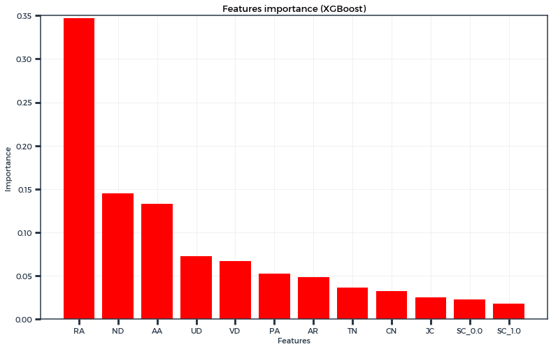
Tree-based boosting algorithms also provide “feature importance”, and an interesting fact here is that there seems to be a correlation between the feature importance of a similarity indice and its prediction quality :

Resource Allocation was the “most important feature” according to this graph, and also as we saw previously, the best unsupervised method. It is quite similar to the Adamic-Adar index, with the only difference being the log at the denominator. In that regard, this may make RA more discriminating than AA as it penalises more the common neighbors which have many neighbors themselves.

Discussion and Future Work

From what we saw there, using a supervised method which combines unsupervised methods seems to be more efficient. This goes on to confirm Kolja Esders’s conclusions as well as our own past experience when working with networks.

This was an “easy” network as we got really high AUC scores, but depending on the complexity and noise in the graph you are working on, this can be more or less difficult to predict accurately future links. The gap between supervised and unsupervised scores can also widen with complex networks.

We decided to use the XGBoost algorithm but it is of course possible to use any other Machine Learning algorithm, so you can try to reproduce this experiment with your favourite binary classifier ! Data processing has been realised using the Networkit library, so you will need it (find more here).

As we never settle for what we possess, the aim in the future would be to perform even better predictions. Building and adding new features to the model may help improve the performance as it would add information. Scaling data before feeding the model could also slightly improve the performance.

And this is how it ends ! We hope that you enjoyed this journey with us through the link prediction problem in a large-scale network. As the code and data are available in addition to this paper, feel free to reproduce this experience and even improve it if you can ! Thank you for your attention.