Adversarially generated Julia sets

I thought I’d follow up my first article/tutorial about Julia, by showcasing another side of the language’s ecosystem, libraries for machine learning.

Namely, I’ll be displaying Knet and AutoGard, by implementing an image generating adversarial network. For the sake of continuity, I will use the Julia set generator we had in the last articles. We’ll feed the images to this GAN and try to get it to generate its own fractal~ish patterns.

If you don’t know what a GAN is, I suggest you just go read the original whitepaper, it’s one of the easiest and most interesting reads as far as machine learning papers go.

Assuming you don’t have the time to do that, but know some basic machine learning concepts, here’s a quick rundown.

A GAN is essentially two models, one that generates, let’s call it G, and one that discriminates (i.e classifies), D. The goal of D is to differentiate examples from a training data from “fakes”, the goal of G is to produce fakes images that fool D.

Getting started

First, we need to import and modify the code from the previous article, in order to make it generate and n dimensional matrix, with differing Julia sets as its rows. This matrix will server as our real examples for training the discriminator. Also, we need to install the dependencies for this model, namely Knet (which includes AutoGard) and Plots + GR for image generation.

Next, we’ll include our dependencies and initialize the plotting backend. More importantly, however, we’ll also define a variable called atype here, our first use of Knet.

If our machine has any GPUs, we can use the type KnetArray, which will, in turn, cause certain algebraic operations on that a array to be executed on the GPU using OpenCl code. If you don’t have any GPUs at your disposal, atype is set to a normal Julia array, and everything is executed on the CPU.

I’d like to note here, that you can realistically run this model on a CPU, I personally ran them on my laptop, on an i5 kabylake mobile CPU.

The model

Now that that’s out of the way, let’s look at the code that will generate all of this stuff. This model is based on this repository, written by Ekin Akyürek, so shoutouts to him.

Note: After writing this, I was informed by Ekin that he actually wrote a blog post about this GAN model, before I had written this one. I encourage you to go checkout his blog.

First, we must create a function to actually build our networks, in this case, some basic multi-layer perceptrons. This essentially amounts to initializing a bunch of vectors (the weights and biases) with zeros or random small values.

Next, we’ll define a simple function to do the forward propagation through our models. This function is generic and can be used with any of the models we define.

The function takes two arguments, W is an array of vectors, with the odd index elements being the weights and the even indexed elements the biases, X is the vector of input features. It also takes an optional argument, which represents the dropout probability for any given value in our vector of weights.

Ok, here’s where we see how the libraries really come together to produce some beautiful code. Which is almost indistinguishable from the actual equations we’d write down to define this model. This is the part of our code where we define our loss functions.

Next, we need some auxiliary code, to help us save the images and to produce the noise which the generator will use as input, in order to introduce randomness in the images it generates. 𝞗 is a dictionary which will just use to carry around various information.

The final piece of this puzzle is a function that will take some data and train our models several time. The essential part is calling the update! macro, this takes the weights vector for the respective model, its gradient (generate by AutoGrad) and an optimizer.

In this case we use Adaptive Moment Estimation, but we could have just as well used SGD, AdaGrad or just simple averaging for our optimizer.

With this information, update! will adjust the weights of our models, in order to try and minimize their loss functions, a process also known as backwards propagation.

Keep in mind the loss functions are interdependent, in an ideal model there should be some balance between the losses of D and G, that is to say, they should have a similar value and never converge to zero.

We’ll define a function that will save the images generated during various epochs and print out the losses for both models in each epoch.

Let’s combine all the pieces together in our main function. This simply consists of defining various hyperparameters and the shape of our network, then running the training function.

Now, we just need to generate some julia sets, feed them as the input data to our model, and watch the pretty images being created.

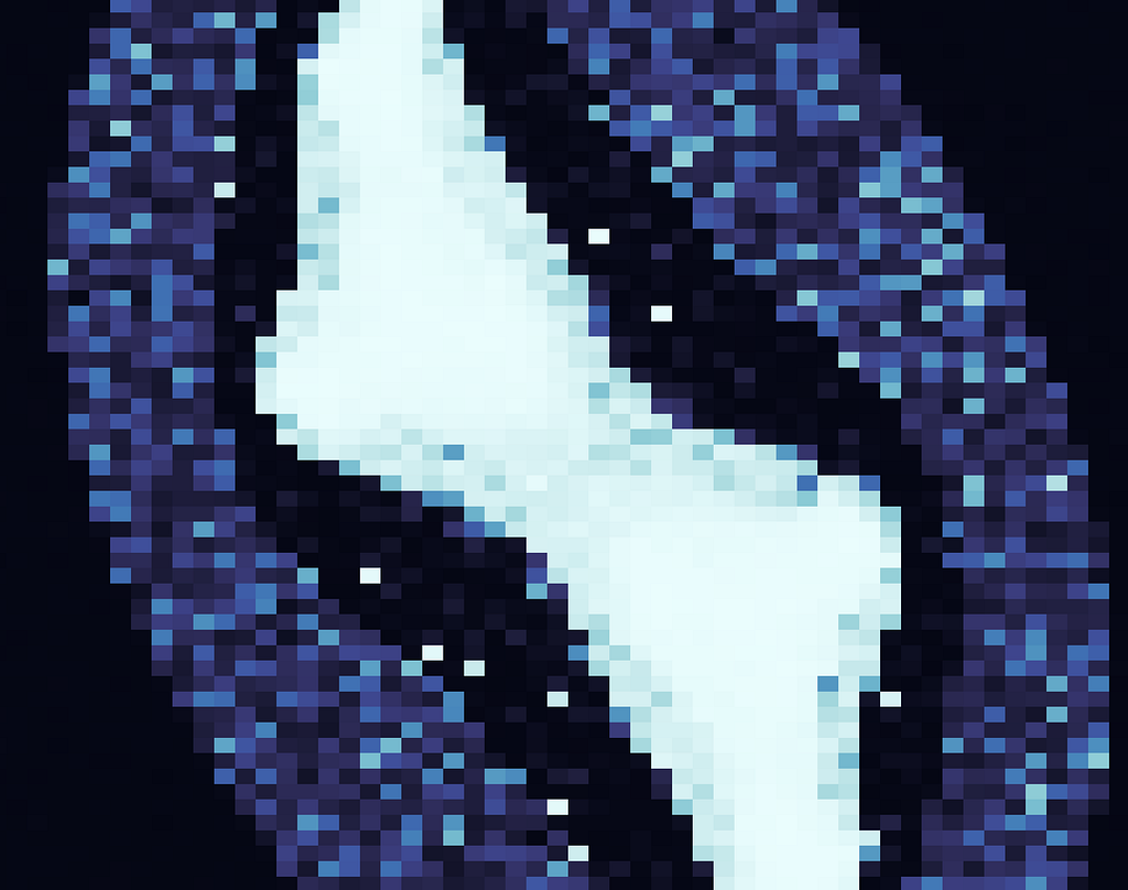
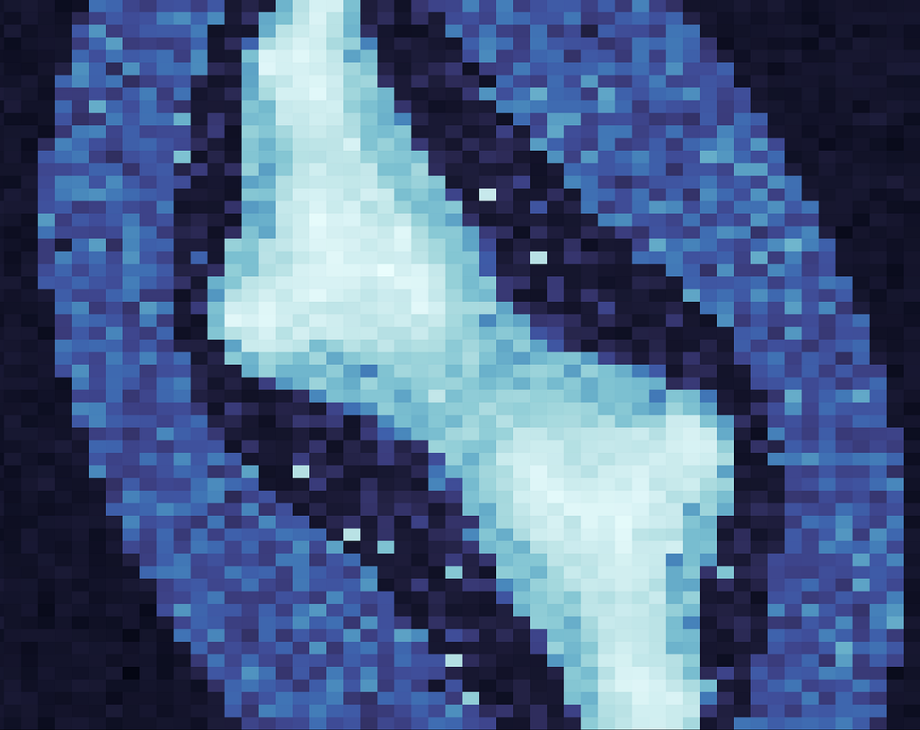
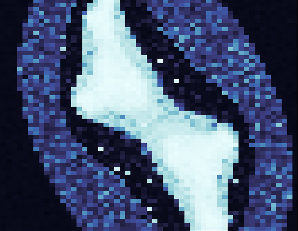
Using various training samples and sizes, here’s some images I’ve managed to generate using this.

Keep in mind, that there’s some element of randomness to the above code, and you can easily slip into a situation where either the G or the D loss converges to zero. Meaning that either the discriminator is unable to distinguish between images, resulting in no improvements to our generator or the discriminator gets “too good” to ever be fooled by our generator, again, resulting in no improvements to our generator.

Adjusting the various hyperparameters. This is where the hard and expensive part of machine learning would come in, where models have to be tuned through a combination of theory, intuition, luck and trial&error.

Obviously, this model doesn’t have recurrent or convolutional layers, which are a staple of most modern neural networks, especially when dealing with images.

However, if you dig a bit into Knet’s docs, I think you’ll find that adapting this model to use a CNN or a LSTMN won’t be that hard.

The beauty of Knet is that is offers a very nice balance between low level primitives and higher level abstractions, making it very useful if you need models that are somewhat unique. The other amazing thing about it, is its performance when compared to leading frameworks in this domain, such as MXnet and Tensorflow.

Adversarially generated Julia sets was originally published in Hacker Noon on Medium, where people are continuing the conversation by highlighting and responding to this story.