The Whitepaper for Portfolio Rebalancing in Crypto

Rebalancing is a growing strategy in the crypto space. Since the release of the Shrimpy application, we have been leading the industry in portfolio rebalancing by creating the most robust platform in the market. During the process of developing our rebalancing services, we acquired a unique prospective that has helped us better understand how rebalancing functions in the crypto space. To help facilitate the transfer of this research into the public domain, we have compiled a whitepaper titled “Portfolio Rebalancing for Cryptocurrency”. This research will lay the foundation for creating a more generalized rebalancing strategy for cryptocurrency. As we continue to expand our research, the whitepaper will be updated accordingly.

Download the whitepaper here.

Introduction

Portfolio rebalancing is a strategy that has been used by investors in the traditional investment markets for decades. However, this simple investment technique has been slow to integrate as a standard for cryptocurrency portfolios. In the following sections, rebalancing will be examined in critical detail.

Portfolio rebalancing is the act of realigning assets in a portfolio back to their target allocations. As the market moves, assets in a portfolio will deviate from their desired percent allocation. Returning to the target allocations requires assets to be bought and sold. This process is called rebalancing.

The target allocation weightings for each asset in a portfolio is determined by the investor when they are constructing a portfolio. These weightings are simply the percent of each asset that should be represented as part of the total value of the combined portfolio. In the case of cryptocurrencies, an asset can be defined as any individual coin or token. When it is time to rebalance, the assets are traded such that the value held in each asset is once again equal to the percentages that were originally specified.

A practical example of this strategy would be if there was a portfolio of 4 different cryptocurrencies. After studying the market, the investor determined that the optimal allocations for each asset in their portfolio was an equal 25% stake in their portfolio. This would mean at the end of each rebalance, the portfolio would consist of 25% in each of the 4 assets. The value of each asset should be converted to a single common value, such as BTC or a fiat currency, so the different assets won’t be evaluated based on quantity, but value. Therefore, if you had $100 total between these four assets, you would have $25 in each after a rebalance took place.

Common Rebalancing Strategies

There are two primary rebalancing strategies which need to be examined. These are periodic rebalancing and threshold rebalancing. While they differ in the reason for why the rebalance was triggered, they both result in assets being bought and sold to realign with the target allocations. Although threshold-based rebalancing is a common strategy, the major topic of discussion throughout this paper will be focused on periodic rebalancing.

Periodic

Figure 1: Simple illustration depicting how periodic rebalancing takes place at specific times. After 24 hours, the allocations are not equal, so a rebalance will make them equal once again.

The simplest of these strategies is periodic rebalancing, which uses a fixed amount of time between each rebalance. This fixed amount of time is called the “rebalance period”. The rebalance period for cryptocurrencies is often far shorter than other asset classes, due to rapid price fluctuations. An example would be selecting a rebalance period of 1 day. In this scenario, a rebalance would occur every day at the same time.

Threshold

Figure 2: This demonstrates a threshold rebalance when a portfolio reaches a 10% deviation. Notice the difference between the green and the blue allocation is 10%. This gap between the two allocations triggers a rebalance.

Rebalancing based on allocation tolerance bands examines the drift of the allocations relative to each other. By relating assets to each other, the variance between each asset is tracked over time. So as the percent allocation of individual assets drift apart, a rebalance takes place when the difference between any two assets crosses a threshold. For example, with a band that is +-5%, if one asset represents 5% more or less of the entire portfolio than it should, the portfolio is rebalanced. Imagine the situation previously discussed where a portfolio had 4 different coins that each held 25% of the portfolio value. In this method, a rebalance would happen as soon as one of those assets consumes less than 20% or more than 30% of the portfolio value. However, this also means that if all the coins in the portfolio are increasing or decreasing in value together, without changing their percent representation in the total portfolio, then no rebalance takes place.

Portfolio Rebalancing Debt Resolution Algorithms in Crypto

This section will detail some of the complexities involved with portfolio rebalancing for cryptocurrencies. Theoretically, rebalancing should be simple, but there are complications that arise based on restrictions that are imposed by exchanges. One of these restrictions is that limit orders commonly have minimum trade requirements. These minimums vary between exchanges, but each result in situations where target allocations cannot be reached. This occurs when the trade necessary to reach a target allocation is less than the minimum trade requirement.

The act of buying more of an asset which needs funds to reach its target allocation is called “debt resolution”. The process of selling an asset which performed well over a period and has a larger allocation than the target allocation is considered “taxation”. Taxing the assets which performed well so they match their target allocations is generally easy, paying the debt out to the remaining assets is more complicated. There are cases where debt cannot be paid. Whether this is a result of a taxed asset not meeting the minimum requirements to make a trade or exchange errors, it doesn’t matter. The result is a situation where more debt is owed than what is available to pay.

Unless otherwise specified, each algorithm will assume trades happen through BTC. This means there will be two discrete steps. First, all assets which have a larger percent allocation than their target allocations will be taxed. This taxation happens by selling the asset for BTC. Second, debt will be paid to each asset which has a smaller percent allocation than their target allocation. Payment will be made from the pool of BTC that was collected during the taxation step.

Constructing algorithms to address this issue should meet the 4 following requirements:

Fairness: The fairest instance is not picking between two assets. This means if there are only enough funds to make one trade, the fairest option is to pick neither. (however, this may not be desired from the user standpoint)

Deterministic: The algorithm should be consistent. It should work every single time. Every reachable state should be predictable.

Usability: An algorithm can be fair and deterministic, but not usable. The algorithm needs to be usable and desirable. It should produce results that the user wants to see.

Economical: Any method used shouldn’t require excessive trades to fit one of the previous requirements. The algorithm should optimize for the smallest amount of fees possible.

Share based debt resolution

Share based debt resolution is an algorithm that attempts fairness in results. The way this solution works is by divvying up the shares by calculating the percent debt held by each asset. For example, let’s say the total debt is 100 BTC, however only 90 BTC is available for payment. This means 90 BTC needs to be divided among 100 BTC of debt. The fairest way to do this is to pay out 90% of the debt that is owed to each individual asset. Instead of satisfying 100% of any assets debt, they will only get 90% of their debt paid.

This is the fairest and most deterministic algorithm. No decisions are made that prioritize a single asset or trade. The issues come from usability and economical decisions.

One issue with this solution is that it is rare to be able to pay out 100% of the debt that is owed. Since this is a rare occurrence, it will be rare to have every asset reach its target allocations. As a result, this algorithm may be less desirable for some users who wish to have as many assets reach their target allocations as possible. In the other sense, this algorithm may be more desirable for some users since this technique is completely unbiased. It does not attempt to anticipate which asset the user would prefer to buy.

Largest debt first resolution

The largest debt first resolution algorithm focuses on paying off the largest debt first. The reasoning behind this algorithm is that the assets which have the largest debt are the furthest from their target allocations. In this sense, it makes sense that the algorithm should satisfy the assets which are furthest from the users desired allocations first.

Let’s examine the same situation that was examined above. Imagine you only have 90 BTC but have 100 BTC of debt to pay. With this algorithm, you will pay the assets which are furthest from their target allocation first. This may result in a single asset getting 90 BTC if they are far enough away. Then, there is 0 BTC left to pay the remaining assets.

While this strategy will likely make sense to some users, it is assuming that the user would want the asset with the largest debt to be paid first. This may not be the case. Since it is an unfair algorithm, this results in assumptions that may not be desirable from the user’s prospective.

Path of Least Resistance Debt Resolution

The path of least resistance debt resolution is slightly different than the previous algorithms. This technique is only available for a subset of asset pairs and bypasses the BTC pool that is collected for debt pay out by other assets. The path of least resistance refers to trading pairs that connect assets directly together, so they don’t need to be traded through BTC during a rebalance. An example of one of these pairs is XRP/ETH on Binance. If a portfolio contains both XRP and ETH, it has an opportunity to trade directly between these two assets without first trading to BTC.

The path of least resistance is always considered the path which results in the largest amount of the resulting asset. So, this considers fees, spread, and slippage to maximize the final asset amount. Given the scenario which two assets are present in the portfolio which are also a pair, they can be evaluated and paid off first given they are the path of least resistance.

The path of least resistance debt resolution can further be generalized to include all trades that result in the smallest spread, slippage, and fees. This results in maximizing purchase power of the portfolio for those assets which are considered cheap to acquire.

The resistance can then be calculated for each asset based on the following criteria:

• # of trades, where higher increases resistance
• % spread, where higher increases resistance
• % slippage, where higher increases resistance
• % fees, where higher increases resistance

Putting it all together

Once these strategies are understood, it’s possible to put them all together to create a rebalancing algorithm which is fair, deterministic, usable, and economical. This is done by performing each of these strategies at different stages.

First, the economical strategy of fulfilling the path of least resistance will be completed. This should be done before any assets have sold to BTC.

Second, the fairest strategy should be used to distribute the BTC that was collected for debt distribution. This allows the spread of debt across all assets which require payment. However, during this process, there may be trades which are smaller than the minimum trade limit if the deviation for some assets are small.

Third, the usable strategy of largest debt first should be used to distribute the BTC which was left over from the previous step. This allows each asset to get as close as possible to the target allocation.

This staged strategy is deterministic which provides a comfort in predictability for how the algorithm will behave during rebalances.

Common Rebalancing Scenarios

The cryptocurrency market presents countless situations which could be evaluated to understand how rebalancing behaves under varying conditions. In this section, several common situations will be constructed to highlight some of the typical cases. Although there are numerous other situations, the scenarios discussed here can be combined in ways to understand nearly any situation.

Pump and Dump

Pump and dumps have been a hallmark of the crypto market. This is when a sharp increase in value is followed by a sharp decline in value for an asset. The result is a return to the original price.

Figure 3: This graph illustrates a pump and dump. The white line is the price of a single asset in a portfolio. The orange line is the value of the portfolio if the HODL strategy is used from beginning the end. The blue line is the value of the portfolio if a rebalance was performed at the white dot.

HODL

The pump and dump examined in this scenario is defined by an initial and ending price that is equal in value. As a result, HODLing through the entire rise and fall would net no portfolio value change.

Rebalance

Pump and dumps provide an opportunity for rebalancing to capture returns for the portfolio. When rebalancing, the excess value generated by the deviating asset is shaved off and spread into other holdings. Since the price of the volatile asset returns to the original value, the net result of a rebalance anywhere along the pump or dump curve is a positive return for the portfolio.

Evaluation

Pump and dumps present an opportunity for rebalancing to increase the total holdings of a portfolio. These same opportunities are not available for portfolios which simply HODL through a pump and dump.

Flash Crash and Recovery

This next example will investigate the behavior of a flash crash and recovery which results in an ending value which is the same as the initial value. This is therefore defined by a sharp value decline followed by a sharp increase in value to return to the original price.

Figure 4: This graph illustrates a flash crash and recovery. The white line is the price of a single asset in a portfolio. The orange line is the value of the portfolio if the HODL strategy is used from beginning the end. The blue line is the value of the portfolio if a rebalance was performed at the white dot.

HODL

The results of HODL for this situation are the same as the pump and dump scenario. Since the beginning and ending price are both the same value, HODL will result in no change of value for the portfolio.

Rebalance

Rebalancing can capitalize on these flash crashes to result in a net positive increase in portfolio value. When rebalancing, the deviating asset is bought while it’s cheap. Since the price of the asset returns to the original value, the net result of a rebalance anywhere along the pump or dump curve is a positive return for the portfolio.

Evaluation

Catching flash crashes with rebalancing can increase the value of a portfolio. This opportunity is not available to portfolios which use the HODL technique.

Sideways Movement

The next situation is a simple sideways movement which takes place for a prolonged period. During this time, there are typically micro fluctuations, although the total value of the portfolio remains relatively flat.

Figure 5: This graph illustrates prolonged sideways movement in the market. The white oscillating line is the price of a single asset in a portfolio. The orange line is the value of the portfolio if the HODL strategy is used from beginning the end. The blue line is the value of the portfolio if a rebalance was performed at the white dot.Figure 6: This graph illustrates prolonged sideways movement in the market. The white oscillating line is the price of a single asset in a portfolio. The orange line is the value of the portfolio if the HODL strategy is used from beginning the end. The blue line is the value of the portfolio if a rebalance was performed at each white dot.

HODL

When examining this case, the results of a portfolio which uses the HODL strategy is the same as those for pump and dump. There should be no net change in portfolio value. This means from the beginning to the end of these micro fluctuations, there is no increase or decrease in asset holdings.

Rebalance

In figure 5, one asset in the portfolio depicted by the white line reduces in value towards the white dot. At this time, the portfolio is rebalanced and the asset experiences accumulation. Then, when the asset increases in value back to the base line, an increase in portfolio value is observed. This situation is present whether the rebalance happens at the valleys or peaks of these fluctuations. When the value of an asset returns to its previous value, it results in a net increase in value for rebalancing.

In figure 6, continuous rebalances are examined throughout the period of prolonged sideways movement. Rebalancing throughout this situation results in a compounding affect. Continuing to rebalance during each peak and valley causes the value of the portfolio to constantly climb.

Evaluation

Sideways movement presents a possibility for rebalancing to capitalize on small fluctuations in asset value. Long periods of sideways movement can result in increases in portfolio value. In addition, rebalancing frequently can result in a compounding affect which boosts performance even further.

Slow Death

The slow death is when a single asset continues to decline in value. Over the entire period, it continues to decrease in value.

Figure 7: This graph illustrates a slow death. The white line is the price of a single asset in a portfolio. The orange line is the value of the portfolio if the HODL strategy is used from beginning the end. The blue line is the value of the portfolio if a rebalance was performed at the white dot.

HODL

HODLing an asset which is having a slow death results in a net decrease in total portfolio value. However, this slow death does not affect the value of any other holding. So, while the total value of the portfolio is decreasing, the subset of the portfolio which excludes the asset which is having a slow death, does not have any decrease in value.

Rebalance

Rebalancing into an asset which is having a slow death decreases portfolio value. In addition to the value of the individual asset declining, it is also declining the value of the rest of the assets in the portfolio as well. So, this means that both this individual asset as well as the rest of the portfolio is bleeding.

Evaluation

This is an undesirable situation to be in when rebalancing. Continually rebalancing into a dying asset will drag the entire portfolio down with it. Maintaining a diverse portfolio along with periodic monitoring of assets mitigates this risk. The smaller the percentage of the total portfolio that a single asset holds, the smaller the risk.

Slow Take Off

As slow take off is when a single asset continuously increases in value. Over the long term, it maintains a generally upward trend.

Figure 8: This graph illustrates a slow climb. The white line is the price of a single asset in a portfolio. The orange line is the value of the portfolio if the HODL strategy is used from beginning the end. The blue line is the value of the portfolio if a rebalance was performed at the white dot.

HODL

HODLing an asset which is slowly increasing in value results in a net increase for the portfolio. This slow incline has no effect on the rest of the portfolio, so the value increase from this asset is directly proportional to its own value increase over time.

Rebalance

Rebalancing an asset which is constantly increase results in shaving off profits and dumping them into the rest of the portfolio. Since this instance is discussing the behavior of a single asset, this would result in a dampening effect on the value increase for this single asset.

Evaluation

Steadily increasing asset value has advantages for both rebalancing and HODL. HODL generates larger returns if the rest of the portfolio value remains stagnant. The reason for this is that profits won’t be taken from the succeeding asset. In the other case, rebalancing has an advantage because a steady increasing asset that always wins is far rarer than many investors believe in the crypto market. This means a more typical case is one asset grows in value, but the next time it is a different asset that has great growth. Given that case, it would be better to shave off some of the profits from one asset since the next time may see a rise in a different asset.

Sharp Decline

A sharp decline is the case where the value of an asset drops quickly and then stabilizes to a new baseline value.

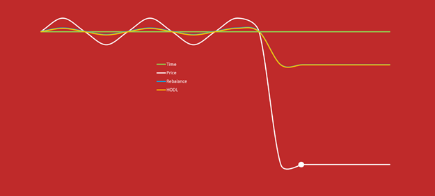Figure 9: This graph illustrates a sharp decline and then stabilization. The white line is the price of a single asset in a portfolio. The orange line is the value of the portfolio if the HODL strategy is used from beginning the end. The blue line is the value of the portfolio if a rebalance was performed at the white dot.

HODL

HODL of an asset which has a sharp decline simply results in the reduction of portfolio value directly proportional to its own value decrease over time.

Rebalance

The results for this situation are the same as those of HODL. While the single asset crash resulted in a net decrease for the portfolio, a rebalance at the dot does not introduce any additional loss in funds. Rebalancing anywhere along the decreasing line before the dot would result in additional loss (See “Slow Death”).

Evaluation

Both rebalancing and HODL perform the same in this instance when looking at the complete portfolio value. Rebalancing at the dot will accumulate more of the asset which had a sharp decline, however, the stabilizing price afterwards means no additional loss in portfolio value is observed.

Sharp Jump

Sharp jump is the situation where a single asset quickly increases in value until it reaches a new baseline value.

Figure 10: This graph illustrates a pump and then stabilization. The white line is the price of a single asset in a portfolio. The orange line is the value of the portfolio if the HODL strategy is used from beginning the end. The blue line is the value of the portfolio if a rebalance was performed at the white dot.

HODL

HODL of an asset which has a sharp rise simply results in the increase of portfolio value directly proportional to its own value increase over time.

Rebalance

The results for this situation are the same as those of HODL. While the single asset pump resulted in a net increase for the portfolio, a rebalance at the dot does not introduce any additional gain in funds. Rebalancing anywhere along the increasing line before the dot would result in underperforming when compared to HODL (See “Slow Take Off”).

Evaluation

Both rebalancing and HODL perform the same in this instance when looking at the complete portfolio value. Rebalancing at the dot will redistribute some of the gains observed during the sharp incline, however, the stabilizing price afterwards means no additional gain in portfolio value is observed.

Rebalancing Backtests

A backtest is the process of using the trade data from an exchange to simulate how a strategy would have performed over a given period. This is often used to test the viability of a strategy by running it through these large data sets. The following sections will detail the constraints which were used when performing the backtests.

Backtest Setup

Trades & Data

A complete year of market data was collected from exchanges between May 4, 2017 to May 3, 2018. This data was used to evaluate the cost of each trade at the exact time a rebalance would have been performed. Additionally, all trades included a .25% fee which was standard for most exchanges at the time of writing. The trading path between each asset was performed by first trading to BTC. So, a trade from LTC to SNT would trade from LTC to BTC and then BTC to SNT. In this instance, both trades incur a .25% fee.

Rebalance Period

Some of the following studies will evaluate the effect of varying the rebalance period. Each section will label the rebalance period of clarity, however the only rebalance periods which will be used are 1 hour, 1 day, 1 week, and 1-month periods.

Portfolio Size & Allocation

At the start of each backtest, the portfolio is seeded with a $5,000 initial investment which is allocated across the assets. The number of assets in each portfolio examined in these studies will range from 2-asset portfolios to 40-asset portfolios. In any given study, 2-asset portfolios were determined to be the smallest portfolio that required analysis.

Unless otherwise specified, all allocations were evenly weighted in the portfolio. A portfolio of 5 assets would therefore have an even allocation of 20% per asset.

Asset Selection

To determine which assets would be considered during the process of constructing a portfolio, a cross section of Bittrex and Poloniex was used. On May 3, 2018 each asset which was listed on Poloniex and had 1 year of data was compared to the list of Bittrex assets which also had a year of data. Any asset which was in both lists was included in the pool for asset selection. When a portfolio was constructed, assets were randomly selected from the pool to create a portfolio. Any duplicates were removed and reselected. After each backtest, a new random group of assets was selected for the next backtest. This process was completed 1,000 times for each strategy type and rebalance period.

Evaluations of Rebalance Frequency

2 Asset Portfolio

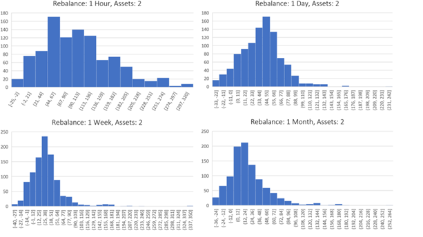Figure 11: This group compares the performance of portfolios which contain two assets but differ by rebalance period. This performance varies from 1 hour (top left chart) to 1 month (bottom right chart). Each histogram incorporates 1,000 backtests, where the x-axis is the percent gain better than HODL. The y-axis is the number of backtests which fell into the performance buckets that are defined on the x-axis. (Example: A backtest was run with a rebalance period of 1 hour and 2 assets in the portfolio. The results of a backtest was a 50% increase over buy and hold. This would mean a 1 is added to the top left chart in the x-axis bucket which has the range of 44 and 67. This process is then repeated until 1,000 backtests have been run.)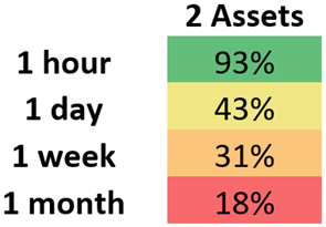Figure 12: This demonstrates the median percent for which rebalancing at varying intervals outperformed HODL for a portfolio which contains two assets.

A 2 asset portfolio represents the simplest option for a portfolio. In this instance, the cryptocurrencies simply trade back and forth to each other during each rebalance period. Figure 11 shows that the shorter rebalancing periods result in a larger spread in performance. There are significantly less outliers for shorter rebalancing periods and the results are consistently higher. As the rebalance period increases, the spread decreases. This results in less variance in results, but a higher observance of outliers. This suggests higher periods produce lower returns consistently, but also produce more sporadic outliers.

The portfolios which used a 1 hour rebalance period outperformed buy and hold by the largest difference of 93%.

4 Asset Portfolio

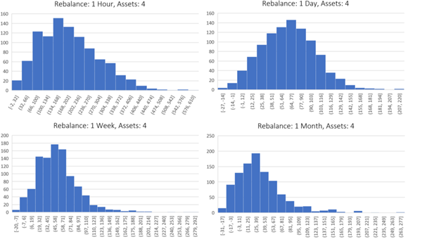Figure 13: This group compares the performance of portfolios which contain four assets but differ by rebalance period. This performance varies from 1 hour (top left chart) to 1 month (bottom right chart). Each histogram incorporates 1,000 backtests, where the x-axis is the percent gain over HODL. The y-axis is the number of backtests which fell into the performance buckets that are defined on the x-axis. (Example: A backtest was run with a rebalance period of 1 hour and 4 assets in the portfolio. The results of a backtest was a 50% increase over buy and hold. This would mean a 1 is added to the top left chart in the x-axis bucket which has the range of 32 and 66. This process is then repeated until 1,000 backtests have been run.)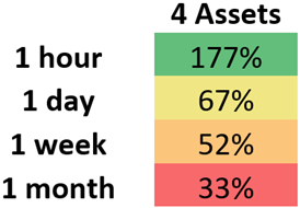Figure 14: This demonstrates the median percent for which rebalancing at varying intervals outperformed HODL for a portfolio which contains four assets.

Continuing the trends from the 2 asset portfolio study, figure 13 demonstrates that shorter rebalance periods have larger spreads in performance in the 4 asset portfolios as well. This results in fewer outliers and a significantly higher median performance than the longer rebalance periods. It can also be observed that the highest performing portfolios all utilized a 1 hour rebalance period. This is even the case when including all outliers.

A period of one hour performed the best with a 177% gain OVER buy and hold.

6 Asset Portfolio

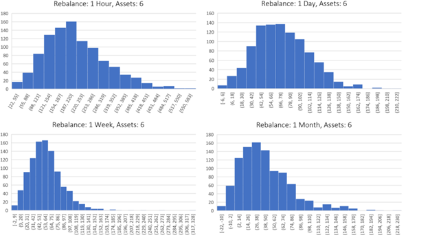Figure 15: This group compares the performance of portfolios which contain six assets but differ by rebalance period. This performance varies from 1 hour (top left chart) to 1 month (bottom right chart). Each histogram incorporates 1,000 backtests, where the x-axis is the percent gain over HODL. The y-axis is the number of backtests which fell into the performance buckets that are defined on the x-axis. (Example: A backtest was run with a rebalance period of 1 hour and 6 assets in the portfolio. The results of a backtest was a 50% increase over buy and hold. This would mean a 1 is added to the top left chart in the x-axis bucket which has the range of 22 and 55. This process is then repeated until 1,000 backtests have been run.)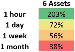Figure 16: This demonstrates the median percent for which rebalancing at varying intervals outperformed HODL for a portfolio which contains six assets.

A 6 asset portfolio continues the trends discussed in the 2 and 4 asset portfolios. This includes the larger spread for shorter rebalance periods and a higher average performance for shorter rebalance periods. Additionally, there appears to be an increasing spread between the 1 hour rebalance period and the 1 month rebalance period as the number of assets in the portfolio continues to increase. This is can be observed by first comparing the 4 asset portfolio to the 2 asset portfolio and then the 6 asset portfolio to the 4 asset portfolio.

A portfolio which contains 6 assets and has a rebalance period of 1 hour outperformed HODL by 203%.

8 Asset Portfolio

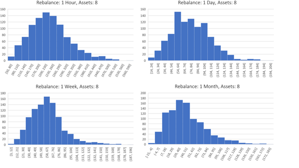Figure 17: This group compares the performance of portfolios which contain eight assets but differ by rebalance period. This performance varies from 1 hour (top left chart) to 1 month (bottom right chart). Each histogram incorporates 1,000 backtests, where the x-axis is the percent gain over HODL. The y-axis is the number of backtests which fell into the performance buckets that are defined on the x-axis. (Example: A backtest was run with a rebalance period of 1 hour and 8 assets in the portfolio. The results of a backtest was a 50% increase over buy and hold. This would mean a 1 is added to the top left chart in the x-axis bucket which has the range of 50 and 80. This process is then repeated until 1,000 backtests have been run.)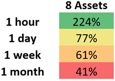Figure 18: This demonstrates the median percent for which rebalancing at varying intervals outperformed HODL for a portfolio which contains eight assets.

An 8 asset portfolio continues the trends discussed in the 2, 4, and 6 asset portfolios. This includes the larger spread for shorter rebalance periods and a higher average performance for shorter rebalance periods. Additionally, there is only one histogram in this study of 8 asset portfolios that contained results which performed worse than HODL. This can be seen in the bottom right chart which represents the portfolios which used a 1 month rebalance period.

The median 8 asset portfolio which rebalanced every 1 hour outperformed HODL by 224%.

10 Asset Portfolio

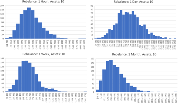Figure 19: This group compares the performance of portfolios which contain ten assets but differ by rebalance period. This performance varies from 1 hour (top left chart) to 1 month (bottom right chart). Each histogram incorporates 1,000 backtests, where the x-axis is the percent gain over HODL. The y-axis is the number of backtests which fell into the performance buckets that are defined on the x-axis. (Example: A backtest was run with a rebalance period of 1 hour and 10 assets in the portfolio. The results of a backtest was a 50% increase over buy and hold. This would mean a 1 is added to the top left chart in the x-axis bucket which has the range of 44 and 72. This process is then repeated until 1,000 backtests have been run.)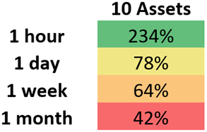Figure 20: This demonstrates the median percent for which rebalancing at varying intervals outperformed HODL for a portfolio which contains ten assets.

The 10 asset portfolio results continue the trends discussed in the 2, 4, 6, and 8 asset portfolios. This includes the larger spread for shorter rebalance periods and a higher average performance for shorter rebalance periods. Additionally, only 10 portfolios out of 4,000 performed worse than HODL if rebalanced at least 1 time each month. This means randomly selecting a portfolio of 10 assets and rebalancing at least once a month results in a 99.75% chance of outperforming buy and hold over the last year.

The median performance for a portfolio with 10 assets and a rebalance period of 1 hour was 234% BETTER than HODL.Complete Comparison

Collecting the results from the previous 5 sections generates a 4 x 5 grid that illustrates the performance of each portfolio and rebalance period. Since the upper bound on most graphs is much higher than the lower bound, the median value is used to prevent a large skew. This also means that 50% of the portfolios were above and 50% of the portfolios were below this value. So, if assets were randomly selected to construct a portfolio, there was a 50% chance of performing better than the listed value.

Also, the listed value is the percent gain over buy and hold. So, a value of 10% would mean rebalancing performed 10% BETTER than HODL.

Figure 21: The median performance demonstrates that the higher the rebalance period with the higher number of assets presents the highest gains for rebalancing. Each value represents a percent increase OVER buy and hold. That means a value of 18 means the median of that group performed 18 percent BETTER than buy and hold. This demonstrates, even the absolute worst case performs better than by and hold, even after considering taxes.

Two major conclusions can be drawn from this grid. First, there is a correlation between the rebalance period and performance over the last year. As the rebalance period becomes shorter, the performance of the portfolio increases. Second, there is a correlation between the number of assets in the portfolio and the performance. As the number of assets in the portfolio increases, there is an increase in performance. In this study, the best performing portfolios were those that had short rebalance periods and many assets.

Rounding out the comparison, the following histogram includes every backtest that was run for this study. It illustrates the performance difference between rebalance and HODL by including all rebalances and portfolio sizes that were evaluated.

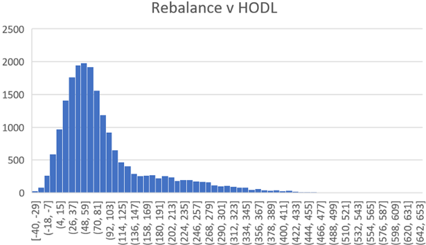Figure 22: Combining all the backtests over all portfolios and rebalancing periods produces a complete picture comparing rebalancing and HODL. This results in a median complete performance of 64%. This means, a randomly selected portfolio size between 2 and 10, a randomly selected rebalance period between 1 hour and 1 month, and a randomly selected portfolio of assets had a 50% chance of performing 64% better than buy and hold if the only difference was rebalancing.The results show a median performance increase of 64% overall portfolio sizes, rebalance periods, and coin selections.

Interpretations

There are two major relations that can be drawn from this study. The first relation is that increasing the number of assets increased the performance of a portfolio. The second relation is that decreasing the rebalance period (increasing rebalance frequency) increased the performance of a portfolio. Therefore, the ideal portfolio was rebalanced frequently and contain numerous assets.

Rebalancing beat HODL by a median of 64%.Studying the Effect of Portfolio Diversity

The following section will investigate the performance impact of increasing the number of assets in a portfolio. The previous section ranged from 2 asset portfolios to 10 asset portfolios. This section will range from 2 asset portfolios to 40 asset portfolios.

HODL

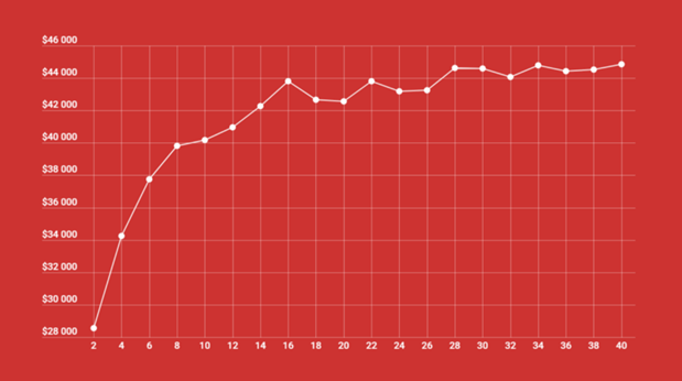Figure 23: This graph shows the results of a $5,000 initial investment that used the HODL strategy for one year. Each data point on the graph is the median return after 1,000 backtests which were run by randomly selecting the number of assets on the x-axis.

This plot shows that HODLing approached an asymptote around $45k after a one-year period. As the number of assets increased past 16, there was a minimal observable difference in value.

1 Month Rebalance

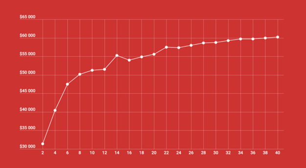Figure 24: This graph shows the results of a $5,000 initial investment that used 1 month rebalances for one year. Each data point on the graph is the median return after 1,000 backtests which were run by randomly selecting the number of assets on the x-axis.

This plot shows that a 1 month rebalance had an apparent asymptote around $60k after a one-year period. As the number of assets increased past ~22, there was a minimal observable difference in value.

1 Week Rebalance

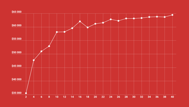Figure 25: This graph shows the results of a $5,000 initial investment that used 1 week rebalances for one year. Each data point on the graph is the median return after 1,000 backtests which were run by randomly selecting the number of assets on the x-axis.

This plot shows that a 1 week rebalance had an apparent asymptote around $65k after a one-year period. As the number of assets increased past ~16, there was a minimal observable difference in value.

1 Day Rebalance

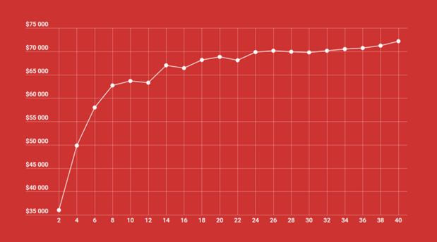Figure 26: This graph shows the results of a $5,000 initial investment that used 1 day rebalances for one year. Each data point on the graph is the median return after 1,000 backtests which were run by randomly selecting the number of assets on the x-axis.

This plot shows that a 1 day rebalance had an apparent asymptote around ~$73k after a one-year period. As the number of assets increased past ~14, there was a minimal observable difference in value.

1 Hour Rebalance

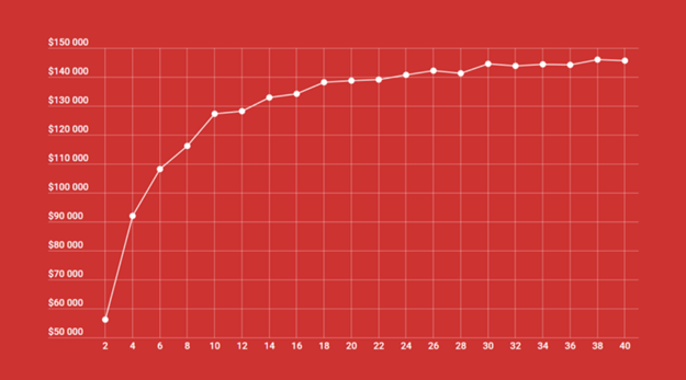Figure 27: This graph shows the results of a $5,000 initial investment that used 1 hour rebalances for one year. Each data point on the graph is the median return after 1,000 backtests which were run by randomly selecting the number of assets on the x-axis.

This plot shows that a 1 hour rebalance had an apparent asymptote around ~$145k after a one-year period. As the number of assets increased past ~18, there was a minimal observable difference in value.

Combined Results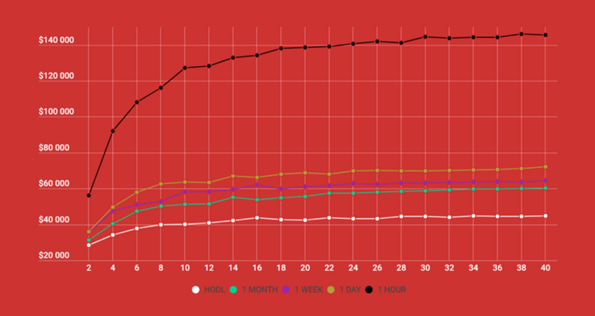Figure 28: This graph shows the results of a $5,000 initial investment that used the strategies as discussed above. Each data point on the graph is 1,000 backtests which were run by randomly selecting the number of assets on the x-axis.

This plot compares the rebalance periods and their performance over the last year. This plot demonstrates that 1 hour rebalances had significantly higher returns than other periods. However, regardless of the strategy, this data suggests that a portfolio ranging from 14 to 22 assets had the highest performance potential per asset over the last year. Above this range adding more assets didn’t provide a large increase in value, although it does provide some benefit. Portfolio sizes below this range resulted in a sharp decline in value.

Optimizing Asset Distribution

Each of the previous backtests were run with an even distribution of assets. The following section will evaluate the performance effect of three different distribution models. These allocation strategies will be the following:

• Even
• Linear
• Exponential

Even Allocation Distribution

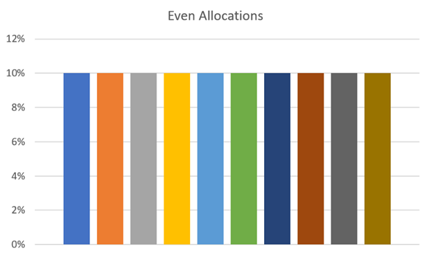Figure 29: This distribution follows an allocation of 10 percent for each asset.

Even distribution means that each asset holds the same weight in the portfolio. A portfolio of 10 assets would result in each asset holding exactly 10% weight in the portfolio. Whenever the portfolio is rebalanced, trades are made to realign the portfolio to match these desired allocations.

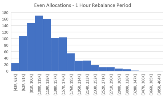Figure 30: This group compares the performance of evenly distributed portfolios which contain 10 assets but differ by rebalance period. Each histogram incorporates 1,000 backtests, where the x-axis is the value of a portfolio after 1 year which had an initial investment of $5,000. The y-axis is the number of backtests which fell into the portfolio value buckets that are defined on the x-axis. (Example: A backtest was run with a rebalance period of 1 hour and 10 evenly distributed assets in the portfolio. The results of a backtest was $200k after one year. This would mean a 1 is added to the bottom right chart in the x-axis bucket which has the range of $195k to $214k. This process is then repeated until 1,000 backtests have been run.)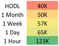Figure 31: These values represent the median portfolio value in USD, 1 year after an initial investment of $5,000. Each value corresponds to their respective histogram displayed above.

Evenly distributed portfolios presented returns that ranged from a $40k median with HODL to a $123k median through rebalancing every hour. In addition to a higher median, rebalancing more frequently also presented a better spread. While the value of portfolios which used the HODL strategy were largely concentrated on the lower end, as observable in the above histograms, frequent rebalances improved the spread by distributing results over a wider range of values and higher performing portfolios. Not only did the median 1 hour rebalance period beat the median HODL, the worst performing portfolio out of over 1,000 backtests in the 1 hour rebalance strategy group beat the median HODL portfolio.

After 1 year, evenly distributed portfolios which rebalanced hourly had a return of 2,360%.

Linear Allocation Distribution

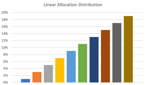Figure 32: This distribution follows an allocation of 1, 3, 5, 7, 9, 11, 13, 15, 17, 19 percent for each asset.

Linear distributions still have a total sum of percentages that equal 100%, but the weights for each asset is uneven. The method in which they are uneven is linear. Since linear can have numerous meanings, linear will be defined as a portfolio with 10 assets that has an allocation distribution of 1, 3, 5, 7, 9, 11, 13, 15, 17, 19 percent per asset. Whenever the portfolio is rebalanced, trades are made to realign the portfolio to match these desired allocations.

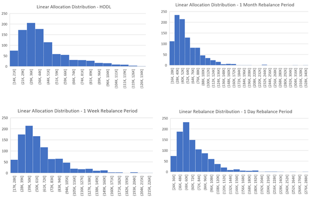
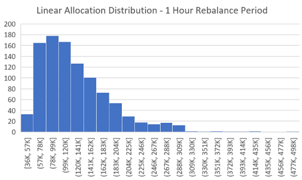Figure 34: This group compares the performance of linearly distributed portfolios which contain 10 assets but differ by rebalance period. Each histogram incorporates 1,000 backtests, where the x-axis is the value of a portfolio after 1 year which had an initial investment of $5,000. The y-axis is the number of backtests which fell into the portfolio value buckets that are defined on the x-axis. (Example: A backtest was run with a rebalance period of 1 hour and 10 linearly distributed assets in the portfolio. The results of a backtest was $200k after one year. This would mean a 1 is added to the bottom right chart in the x-axis bucket which has the range of $183k to $204k. This process is then repeated until 1,000 backtests have been run.)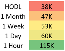Figure 33: These are the median portfolio values for each set of backtests which are detailed in the histograms above.

The results for a linear asset distribution present a decline in returns over a 1-year period when compared to even distributions. The median values saw a decrease ranging from $2k for portfolios which used the HODL strategy, to $8k for portfolios which performed rebalances every 1 hour. The histograms also reveal that linear asset distributions decreased the spread of the results. Instead of a smooth curve, results aggregated at the lower end of this spread. This suggests that not only the median decreased, but there were also fewer high performing portfolios.

After 1 year, linearly distributed portfolios which rebalanced hourly had a return of 2,200%.

Exponential Allocation Distribution

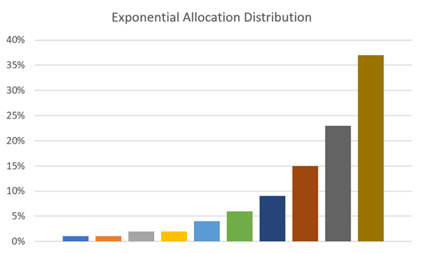Figure 35: This distribution follows an allocation of 1, 1, 2, 2, 4, 6, 9, 15, 23, 37 percent for each asset.

The final method of allocation distribution is the exponential distribution. This method results in one asset holding the lion’s share of the total portfolio value and each asset after that holding a fraction of the previous. In a portfolio of 10 assets, an exponential distribution is defined as a portfolio with an allocation distribution of 1, 1, 2, 2, 4, 6, 9, 15, 23, 37 percent per asset. Whenever the portfolio is rebalanced, trades are made to realign the portfolio to match these target allocations.

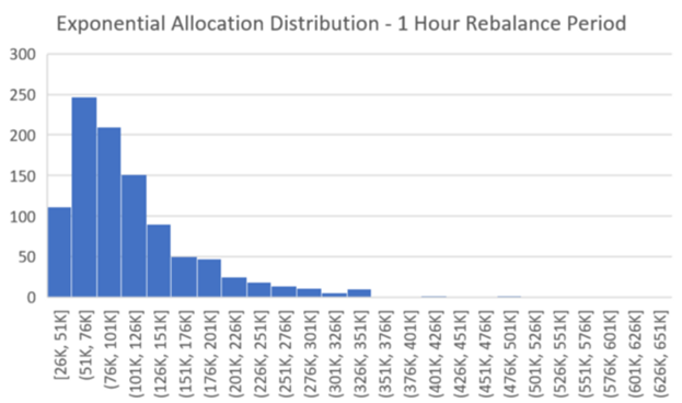Figure 36: This group compares the performance of exponentially distributed portfolios which contain 10 assets but differ by rebalance period. Each histogram incorporates 1,000 backtests, where the x-axis is the value of a portfolio after 1 year which had an initial investment of $5,000. The y-axis is the number of backtests which fell into the portfolio value buckets that are defined on the x-axis. (Example: A backtest was run with a rebalance period of 1 hour and 10 exponentially distributed assets in the portfolio. The results of a backtest was $200k after one year. This would mean a 1 is added to the bottom right chart in the x-axis bucket which has the range of $176k to $201k. This process is then repeated until 1,000 backtests have been run.)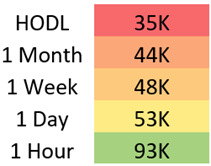Figure 37: These are the median portfolio values for each set of backtests which are detailed in the histograms above.

The results for an exponential asset distribution presented an even larger decline in returns over 1 year when compared to both even and linear distributions. The median values saw a decrease ranging from $3k for portfolios which used the HODL strategy, to $20k for portfolios which performed rebalances every 1 hour. The histograms illustrate this continued trend of declining spread. The results are aggregated at the lower end of this spread, even more than the backtests which explored linear allocation distributions. This suggests both a decrease in median from the linear distribution, as well as a decrease in frequency of high earning portfolios.

After 1 year, linearly distributed portfolios which rebalanced hourly had a return of 1,760%.

Interpretations

Combining all the results from this study, the outcome is a heatmap of how the median portfolio performed over the last year for each of these strategies and rebalance periods.

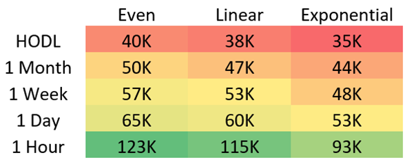Figure 38: These are the median portfolio values for each set of backtests combined across all histograms which were detailed above. Each value represents 1,000 backtests. With a starting portfolio value of $5,000, these median values represent the final value held by the portfolio after 1 year.

This heat map indicates that even distributions with a 1 hour rebalance outperformed non-even distributions over the last year. In fact, the more uneven the distribution of funds, the worse the median portfolio performed.

Evaluation of Market Capitalization

The design for this section was such that assets were divided into 3 categories; large ($70M — $26B), mid ($9M — $69M), and small ($900k — $7.8M) market capitalization. The capitalization ranges were defined by dividing the assets into 3 even groups based on the market cap of each asset on May 4, 2017. During the asset selection phase of the backtest, assets were randomly selected from within each market cap group.

Performance

Four separate groups were evaluated: Large, mid, small, and combined market cap assets. Combined market cap represents all assets regardless of market capitalization.

Large Market Cap

Figure 39: These values represent the total holdings of the median large market cap portfolio after one year. The top left value representing a portfolio which performed no trades over the course of a single year and contained 2 assets. The bottom right represents a portfolio of 10 assets which were rebalanced every 1 hour. Each cell represents exactly 1,000 backtests which were combined to calculate the median.

In this study, large market cap coins consist of assets which fit into the $70M — $26B valuation range. Each valuation was taken on May 4, 2017.

The results of this group indicate there was no observable performance boost through simply increasing the number of assets in a portfolio which used the HODL strategy. However, as the rebalance frequency is increased, the performance increases as well. The largest of these performance boosts were observed with a 1 hour rebalance period.

Rebalancing a large market cap crypto portfolio resulted in up to a 1140% return over a one-year period.

Mid-Market Cap

Figure 40: These values represent the total holdings of the median mid-market cap portfolio after one year. The top left value representing a portfolio which performed no trades over the course of a single year and contained 2 assets. The bottom right represents a portfolio of 10 assets which were rebalanced every 1 hour. Each cell represents exactly 1,000 backtests which were combined to calculate the median.

In this study, mid-market cap coins consist of assets which fit into the $9M — $69M valuation range. Each valuation was taken on May 4, 2017.

Mid-market cap coins demonstrated the highest return of any group over the last year. Not only do they present a strong case for diversifying even when HODLing, they demonstrated impressive growth when rebalanced frequently. One hour rebalances resulted in a 156% increase in portfolio value when compared to HODL.

Rebalancing a mid-market cap crypto portfolio resulted in up to a 3980% return over a one-year period.

Small Market Cap

Figure 41: These values represent the total holdings of the median small market cap portfolio after one year. The top left value representing a portfolio which performed no trades over the course of a single year and contained 2 assets. The bottom right represents a portfolio of 10 assets which were rebalanced every 1 hour. Each cell represents exactly 1,000 backtests which were combined to calculate the median.

In this study, small market cap coins consist of assets which fit into the $900k — $7.8M valuation range. Each valuation was taken on May 4, 2017.

Small market cap coins presented interesting results. HODLing a small market cap portfolio demonstrated the lowest returns of any market cap group over the last year. However, increasing the rebalance frequency provided increased performance improvements. Although HODLing performed worse than large market cap assets, a 1 hour rebalance period resulted in returns greater than large market cap assets.

Rebalancing a small market cap crypto portfolio resulted in up to a 2820% return over a one-year period.

Combined (Any Market Cap)

Figure 42: These values represent the total holdings of the median portfolio after one year. The top left value representing a portfolio which performed no trades over the course of a single year and contained 2 assets. The bottom right represents a portfolio of 10 assets which were rebalanced every 1 hour. Each cell represents exactly 1,000 backtests which were combined to calculate the median.

Combining all market caps provides a general overview of the combined markets. Mixing assets with different market caps into a portfolio creates a middle of the road performance.

Rebalancing a crypto portfolio resulted in up to a 2340% return over the last year.

Interpretations

The results show that mid-market cap portfolios outperformed small, large, and mixed market cap portfolios over the last year. HODLing small market cap portfolios resulted in the worst returns over a 1-year period. Finally, although HODLing a large market cap portfolio outperformed small market cap portfolios, large market cap portfolios underperformed all other portfolio groups when rebalanced frequently.

The Case for Rebalancing

Reducing Market Volatility

Rebalancing is a strategy which can improve the stability of the market. As the market continues to mature, more investors will rebalance their portfolio. So, as the value of assets start to go up, more investors will begin selling the asset, which will bring the price back down. Likewise, when an asset declines in value, these investors will buy the asset which will bring the price back up. This prevents the rapid fluctuations which have been common in the crypto market as larger market forces will be required to move the price of an asset.

Low Maintenance

When compared to most strategies, rebalancing requires a minimal amount of effort from the investor. After setting the initial parameters, there is no required upkeep for the portfolio. Assets can be added or removed from the portfolio periodically based on desire, but this work is typically minimal.

Setting up a rebalancing strategy is also a simple task. To begin, the investor must only select a rebalance period and the asset allocations. Once determined, the rebalance should be performed at the designated interval. Whether performed manually or through a 3rd party service, the strategy will not attempt to time the market. It simply requires buying and selling of assets to realign to the target allocations at the specified interval.

Backtests Demonstrate Promising Results

The previous sections illustrated some of the performance effects that were experienced because of rebalancing over a one-year period. In general, rebalancing a diverse portfolio showed improved returns over the one-year period when compared to HODL. This suggests there may be opportunities for investors to take advantage of rebalancing in the crypto market.

Disclaimer: Backtests examine past performance and do not guarantee future performance.

Conclusions

On the surface, rebalancing is a simple strategy: realign the current allocations with the target allocations. However, digging into the details surfaces complexities that complicate the way rebalances are performed. This whitepaper attempts to illuminate these complexities and provide a foundation for future research.

This whitepaper is in no manner providing investment advice, tax advice, legal advice, or other professional advice. Shrimpy does not recommend, or endorse the purchase or sale of assets, digital or otherwise, or that the reader make any investment or enter into any trade or transaction. Before engaging in any trading or investment activity, the reader should always consult a qualified professional.

Don’t forget to check out the Shrimpy website, follow us on Twitter and Facebook for updates, and ask any questions to our amazing, active communities on Telegram & Discord.

The Shrimpy Team

The Whitepaper for Portfolio Rebalancing in Crypto was originally published in Hacker Noon on Medium, where people are continuing the conversation by highlighting and responding to this story.