DeepMind’s Amazing Mix & Match RL Technique

Mix & Match — Agent Curricula for Reinforcement Learning [ arxiv ]

The Reinforcement Learning Techniques that are used nowadays are very quick and give immediate results for less complex environments using the gradient based policy optimisations.

The Gradient based policies are competitive and not collaborative.

So what if we need long lasting results for more complex environments having agents with complex tasks to perform.

There are many world environment where we do not have the ability to modify the environments and performing Reinforcement Learning on the real world tasks are really time consuming. So to over come that problem this paper tries to solve that issue with the help for Curriculum Learning and Population Based Training.

Before You Start

Curriculum Learning [Paper]To design a sequence of task using transfer learning for an agent to train on, such that final performance or learning speed is improved.Population Based Training for Neural Networks [DeepMind Blog]PBT has the ability to modify the hyper-parameters of the Network while training.

The Main Idea

The main idea behind the Mix & Match paper is to

Generate multiple variants of RL agents where we don’t have the ability to modify task arranged according to training complexity but only use one MIX & MATCH agent constructed by leveraging different agent varying structurally by their policy generation process.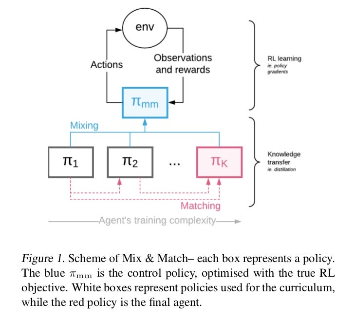

MIX & MATCH Framework

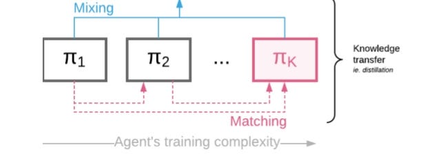
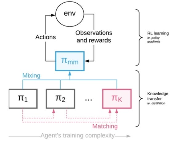
Multiple agents that are arranged in learning complexity (shown above) are treated as one Mix & Match Agent acting with a mixture of policies.

The knowledge transfer (i.e. distillation) is done in such a way that the complex agents are matched with the simpler ones early on.

Mixing Coefficient is controlled such that ultimately complex target agent is used to generate experience.

Method Details

Let’s assume we are given a sequence of trainable agents 1 ( with corresponding policies π 1 , …, π K , each parametrised with some θ i ⊂ θ which can share some parameters)

The aim is to train π K ,while all remaining agents are there to induce faster/easier learning.

Let’s introduce categorical random variable ‘c’ ∼ Cat(1, …, K|α) Probability mass function p(c = i) = α i ) which will be used to select apolicy at a given time:

The point of Mix & Match is to allow curriculum learning, consequently we need the probability mass function (pmf) of c to be changed over time. Initially the pmf should have α 1 = 1 and near the end of training α K = 1 thus allowing the curriculum of policies from simple π 1 to the target one π K.

Now, it should be trained in such a way which maximises long lasting increase of performance and share knowledge together unlike those gradients.

To address this issue we will be using a Distillation-like Cost (D) which will align the policies together.

The final optimisation problem we consider is just a weighted sum of the original L^RL loss (below), applied to the control policy π^mm and the knowledge transfer loss:

Now, let’s understand the Mix & Match Architecture in Steps →

Policy Mixing

Policy mixing will be done by explicit mixing for the sake of variance reduction.

Knowledge Transfer

For simplicity we consider the case of K = 2. Consider the problem of ensuring that final policy (π2) matches the simpler policy (π1) , while having access to samples from the control policy(πmm) .

Same as previous one

For simplicity, we define our M&M loss over the trajectories directly and trajectories (s ∈ S) are sampled from the control policy. The 1 − α term is introduced so that the distillation cost disappears when we switch to π 2 .

Adjusting α (alpha) through training

α is the variable used in the population mass function equation (first equation).

This is the first equation

An important component of the proposed method is how to set values of α through time. For simplicity let us again consider the case of K = 2, where one needs just a single α (as c now comes from Bernoulli distribution) which wetreat as a function of time t.

Online hyperparameter tuning → Since α changes through time one cannot use typical hyperparameter tuning techniques as the space of possible values is exponential in number of timesteps (α = (α (1) , · · · , α (T ) ) ∈ 4 Tk−1 ,where 4 k denotes a k dimensional simplex).

To solve this issue we use Population Based Training (PBT).

Population Based Training and M&M

Population Based Training (PBT) keeps a population of agents, trained in parallel, in order to optimise hyperparameters through time while training and periodically query each other to check how well they are doing relative to others. Badly performing agents copy the weights (neural network parameters) of stronger agents and perform local modifications of their hyperparameters.

This ability of PBT to modify hyperparameters throughout a single training run makes it is possible to discover powerful adaptive strategies e.g. auto-tuned learning rate annealing schedules.

This way poorly performing agents are used to explore the hyperparameters space.

So, we need to define two functions →

eval → which measures how strong a current agent isexplore → which defines how to instigate the hyperparameters.Note: Keep in mind the PBT agents are the MIX & MATCH Agents which is already a mixture of constituent agents.

Now, we should use one of the two schemes mentioned below, depending on the characteristics of the problem we are interested in.

1. If models is having performance improvement by switching from simple to the more complex model, then

a ) Provide eval with performance (i.e. reward over k episodes) of the mixed policy.

b ) For an explore function for α we randomly add or subtract a fixed value (truncating between 0 and 1). Thus, once there is a significant benefit of switching to more complex one — PBT will do it automatically.

2. Often we want to switch from an unconstrained architecture to some specific, heavily constrained one (where there may not be an obvious benefit in performance from switching).

When training a multitask policy from constituent single-task policies, we can make eval an independent evaluation job which only looks at performance of an agent with α K = 1.

This way we directly optimise for the final performance of the model of interest, but at the cost of additional evaluations needed for PBT.

EXPERIMENTS

Let’s test and analyse whether our new M&M method is working correctly in all circumstances. We will now consider 3 sets of Reinforcement Learning experiments which can be Scaled to large and complex action spaces, Complexities of Agents Architecture and Learning Multitask Policy.

In all the process, we initialise α around 0 and analyse its adaptation throughtime.

Note → that even though in the experimental sections we use K = 2, the actual curriculum goes through potentially infinitely many agents being a result of mixing between π 1 and π 2 .

Unless otherwise stated, the eval function returns averaged rewards from last 30 episodes of the control policy.

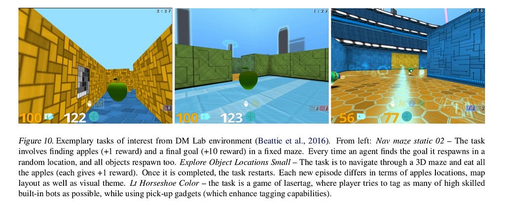
The Environment Suite of DeepMind Lab offers a range of challenging 3D, first-person view based tasks (see, appendix) for RL agents. Agents perceive 96 × 72 pixel based RGB observations, at 60 fps and can move, rotate, jump and tag built-in bots.

1. Curricula Over Number of Actions Used

The action space is complex represented in 6 dimensional vector where two action group are very high resolution (rotation and looking up/down actions) and remaining four are low resolution actions (moving forward, backward or not moving at all, shooting or not shooting etc).

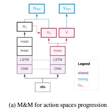
Here, we use 9 actions to construct π 1, the simple policy (Small action space).

Similarly to the research in continuous control using diagonal Gaussian distributions we use a factorised policy π 2 (a 1 , a 2 , …, a 6 |s) := j=1 π̂ j (a j |s), which we refer to as Big action space.

In order to be able to mix these two policies we map π 1 actions onto the corresponding ones in the action space of π 2.

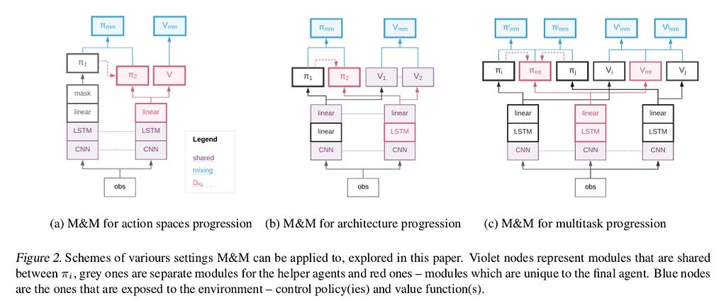
The mixing of values between networks of agents shown in the figure below.

The paper also discussed Shared Head and Masked KL techniques but both are wore than M&M.

RESULTS

We see that the small action space leads to faster learning but hampers final performance as compared to the big action space.

Mix & Match applied to this setting gets the best of both worlds, it learns fast, and surpasses the final performance of the big action space.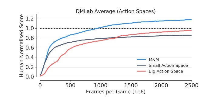FIG: Training in actionspaces experiments.

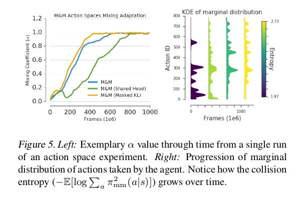
When plotting α through time (Fig. 5 Left) we see that the agent switches fully to the big action space early on, thus showing that small action space was useful only for initial phase of learning. This is further confirmed by looking at how varied the actions taken by the agent are through training.

Fig. 5 (Right) shows how the marginal distribution over actions evolves through time.We see that new actions are unlocked through training, and further that the final distribution is more entropic that the initial one, which means that more entropy leads to more stability.

2. Curricula Over Agent Architecture

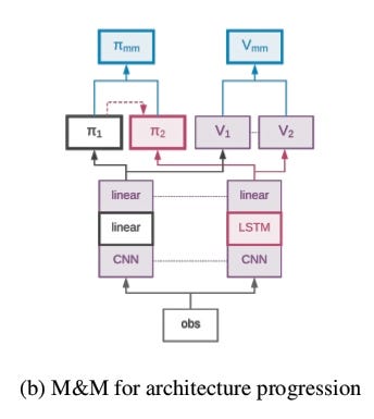
We substitute the LSTM with a linear projection from the processed convolutional signal. We share both the convolutional modules as well as the policy/value function projections.

The experiments are focused on various navigation tasks.

On one hand, reactive policies (which can be represented solely by a Feed Forward policy) should learn reasonably quickly to move around and explore, while on the other hand, recurrent networks (which have memory) are needed to maximise the final performance — by either learning to navigate new maze layouts (Explore Object Location Small) or avoiding (seeking) explored unsuccessful (successful) paths through the maze.

RESULTSFIG 6

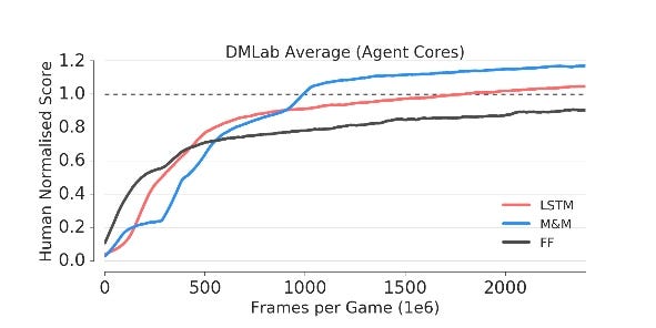
M&M applied to the transition of LSTM and FF, leads to significant improvement in the final performance. But not as fast as FF counterpart.

FIG 7

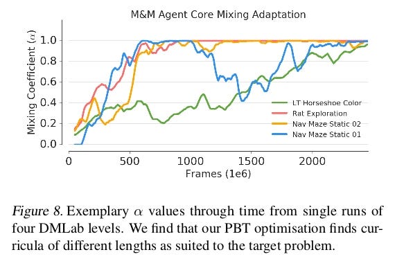
FIG 8 leads to two observations

1. The Green curve switches late to LSTM due to complexity in the level of Game.
2. The model (Blue Curve) has the ability to switch back to the mixture policy if needed.

3. Curricula for Multitask

As a final proof of concept we consider the task of learning a single policy capable of solving multiple RL problems at the same time. The basic approach for this sort of task is to train a model in a mixture of environments or equivalently to train a shared model in multiple environments in parallel.

This type of training can suffer from two drawbacks:

→ It is heavily reward scale dependent, and will be biased towardshigh-reward environments.

→ Environments that are easy to train provide a lot of updates for the model and consequently can also bias the solution towards themselves.

Let’s take a look at the results:

FIG 9

One is Explore Object Locations Small, which has high rewards and a steep initial learning curve (lots of reward signal coming from gathering apples).

In remaining two problems training is hard, the agent is interacting with other bots as well as complex mechanics (pick up bonuses, tagging floors, etc.)

The multitask solution focuses on solving the navigation task, while performing comparitively poorly on the more challenging problems.

To apply M&M to this problem we construct one agent per environment(each acting as π 1 from previous sections) and then one centralised “multitask” agent (π 2 from previous sections). Crucially, agents share convolutional layers but have independent LSTMs.

Training is done in a multitask way, but the control policy in each environment is again a mixture between the task specific π i (the specialist) and π mt (centralised agent).

Since it is no longer beneficial to switch to the centralised policy, we use theperformance of π mt (i.e. the central policy) as the optimisation criterion (eval) for PBT, instead of the control policy.

We evaluate both the performance of the mixture and the centralised agent independently. Fig. 9 shows per task performance of the proposed method. One can notice much more uniform performance —

M&M agent learns to play well in both challenging laser tag environments, while slightly sacrificing performance in a single navigation task.

One of the reasons of this success is the fact that knowledge transfer is done in policy space, which is invariant to reward scaling. While the agent can still focus purely on high reward environments once it has switched to usingonly the central policy, this inductive bias in training with M&M ensures a much higher minimum score.

CONCLISION

Over time the component weightings of this mixture are adapted such that at the end of training we are left with a single active component consisting of the most complex agent. Also,

Improved and Accelerated performance in Complex Environment.Collection of agents is bound together as a single composite whole usinga mixture policy.Information can be shared between the components via shared experience or shared architectural elements, and also through a distillation-like KL-matching loss.

I will be posting 2 posts per week so don’t miss the tutorial.

So, follow me on Medium and Twitter to see similar posts.

Any comments or if you have any question, write it in the comment.

Clap it! Share it! Follow Me!

Happy to be helpful. kudos…..

Previous stories you will love:

• 50 TensorFlow.js API Explained in 5 Minutes | TensorFlow.js Cheetsheet
• TensorFlow 1.9 has Arrived!
• TensorFlow on Mobile: Tutorial
• Activation Functions: Neural Networks

DeepMind’s Amazing Mix & Match RL Technique was originally published in Hacker Noon on Medium, where people are continuing the conversation by highlighting and responding to this story.