A brief overview of Automatic Machine Learning solutions (AutoML)

From mathematical formalism to a description of available solutions (+ Kaggle benchmark)

by Julien Jouganous, Romain Savidan and Axel Bellec (Data Scientists at Cdiscount)

the hyperparameters jungle — Photo by chuttersnap on Unsplash

What is AutoML and why do we need it?

Auto ML is the fact of simplifying data science projects by automating the machine learning tasks. The figure 1 below presents a classical machine learning pipeline for supervised learning tasks.

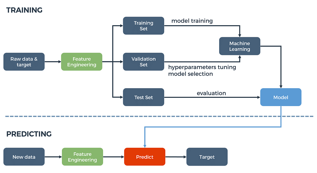Figure 1: A machine learning process.

In the process presented above, several blocks must be tuned to extract most of the predictive power of the data:

First of all, you have to select relevant data that potentially explain the target you want to predict. Once these raw data are extracted, you generally need to process them.

A non-exhausive list of preprocessing steps is given below:

text vectorization
categorical data encoding (e.g., one hot)
missing values and outliers processing
rescaling (e.g., normalization, standardization, min-max scaling)
variables discretization
dimensionality reduction

Last but not least, you have to choose a machine learning algorithm depending on the kind of task you are facing: supervised or not, classification or regression, online or batch learning…

Most machine learning algorithms need parameterization and even if some empirical strategies can help (this article provides guidelines for XGBoost), this optimization is complex and there is generally no deterministic way to find the optimal solution. But that is only the tip of the iceberg as the whole process involves choices and manual interventions that will impact the efficiency of the machine learning pipeline.

Welcome to the hyperparameters jungle!

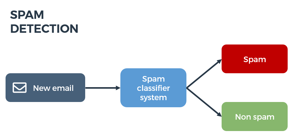
To illustrate this, consider the classical spam detection problem: using the content of emails, you want to predict whether an email is a spam or not. To do that, we have a database with emails tagged as SPAM or NOT_SPAM so this is a supervised binary classification problem.

Figure 2: Spam detection

As machine learning algorithms generally deal with numerical vectors, the first step is to vectorize our emails. We can use a tf-idf approach. But before, we have to tokenize the emails (turn sentences into lists of words). We may also want to apply more advanced text preprocessing such as lowercasing, stemming, lemmatization, or spelling correction.

Now the emails are tokenized and preprocessed, we can vectorize them computing the tf-idf weights but here again the algorithm needs to be parameterized. Indeed, we generally want to specify stopwords, truncate the document frequency range (i.e.remove from the dictionnary rare and/or frequent words), or even include n-grams (sequences of n consecutive words) into our dictionnary.

We have a vectorized representation of our emails. We may or may not want to apply a dimensionality reduction technique such as PCA. We may also want to add other features such as the number of words in the mail, the average word length for example.

It is now time to train our machine learning model but which one will we use?

For this kind of batch supervised binary classification task, we are spoilt for choice: logistic regression, naive Bayes classifier, random forest, gradient boosting, neural nets… We probably want to try and compare some of these algorithms but here let say that we have chosen the random forest. How many decision trees do we need? What is the optimal tree depth? How do we control the leaves granularity? How many samples and features do we want to include in each tree?

Just have a look at the scikit learn documentation to have an overview of the amount of hyperparameters you can tune.

Finally, each component of the pipeline involves choices and parameters that can impact the performances of the algorithm. Auto ML simply consists in automating all these steps and optimizing data preprocessing, algorithm choice and hyperparameters tuning.

Hyperparameters optimization strategies

Mathematical formalism

Consider 𝚨 the possible strategies space. It may sound a bit abstract but let’s just say that each element A ∈ 𝚨 is a parameterization of the machine learning pipeline from the data processing to the model hyperparameters tuning. The auto ML process aims at finding A* such that:

where

and

are train and validation sets obtained via K-fold cross validation and

is the loss for pipeline A trained on training dataset i and evaluated on validation dataset i.

Random search, grid search

The first and simplest tuning approach that may come to mind is just picking randomly several parameterizations of the pipeline and keep the best one. A variant called grid search consists in testing the nodes of a discretization grid of 𝚨. For more details, these algorithms are implemented in scikit learn, here is the documentation.

These Monte-Carlo-like algorithms can be a good starting point for low dimensional problems but, as we saw before, we generally have a consequent amount of parameters to tweak so they will converge very slowly. Moreover, in the grid search case, if optimal strategies are far from the nodes you defined, you have no chance to discover them.

Metaheuristics

To overcome the poor convergence properties of random search, one may want to implement more “clever” algorithms. Metaheuristics are a class of generic optimization techniques based on the exploitation / exploration trade-off and often mimicking biological or physical phenomena. They can be efficient to solve convex and non-convex problems.

Among the tons of metaheuristics, we can mention for instance:

Simulated annealing is a method inspired from annealing in metallurgy that consists in alternating cooling and heating phases to minimize the material enregy modifying its micro structure and physical properties. In analogy, we explore the parameters space to try to minimize the system energy (our objective function). We also introduce the temperature of the material T. At each step, we test a configuration in the neighborhood of the previous one. The higher the temperature is, the more the atoms are free to move and the larger the neighborhood is. Consequently, at the beginning of the process, when T is high, we explore pretty much all the search space and as this temperature decreases, we focus more and more on the areas deemed promising. See here for a more detailled description.
Particle swarms uses a population of candidate solutions (or particles) to explore the space 𝚨. Each particle moves in 𝚨 depending on its current location, its best known past position and the whole population’s best position. The trade-off between exploitation and exploration can be tuned by playing whith the relative importance of these different factors. This paper gives more details about the algorithm and some variants.
Evolutionary algorithms is a family of algorithms inspired by biological evolution. We consider a population of candidate solutions (or individuals) and we apply simplified evolution laws to have them optimize the objective function called fitness. At each step or generation, we select the best (meaning here the fittest) individuals. The next generation is built via the reproduction of these selected individuals. During this step we apply genetic operations: recombination (exploitation) is the process by which the parents features are combined to form children solutions, whereas mutations, introduce random (exploration) perturbations. This way, the average population’s fitness is supposed to improve from one generation to the next and the fittest individual to converge to a good solution of your optimization problem.

Bayesian approaches

Each evaluation of the objective function we try to minimize can be very expensive as we have to train and evaluate a machine learning pipeline. Bayesian optimization provides an efficient method to explore the parameter set and converge quickly to a convenient solution. In short: it helps focus the exploration of the parameter space 𝚨 on promising areas. The figure 3 below (source) gives a simple example in one dimension (in this case, we want to maximize the function):

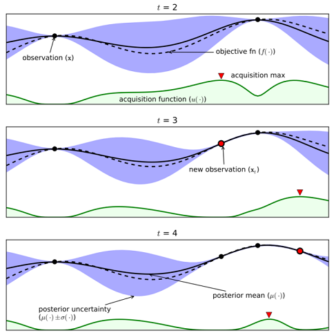Figure 3: Bayesian optimization.

In this example, the objective function f is approximated through a Gaussian Process regression model. This modelling technique provides a probability density function for the values of f based on priors (points where the value of the function is known). This density is represented by the blue area and the mean is plotted in solid line. The distribution is very peaked (small variance) close to observations whereas we are not confident (high variance) with our estimations of f in unsampled areas.

At each step, the new point to explore is selected as the maximum of a function called activation function (the green one). This function synthesizes the a priori knowledge and the uncertainty about the function to optimize. It is high where the predicted objective function is high (or low if we want to minimize f) and where the uncertainty is also high. In other words, it is high where there is a good chance we find better solutions for our optimization problem.

The opposing forces

In this section we provide a non exhaustive list of auto ML solutions currently available. We arbitrarily chose a few summary features to compare them: Is it a open source package? Which backend models implementation and hyperparameters tuning algorithms are used? How many contributors?

These features, when they where available, were gathered in the table below. Note that it is a snapshot of these libraries at the time this article was written.

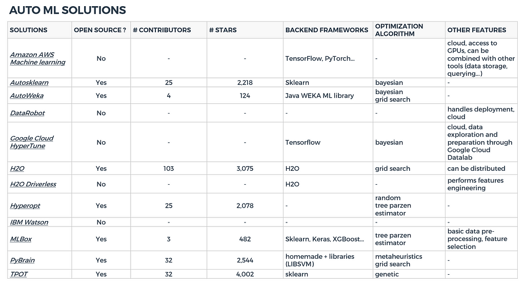Figure 4: AutoML solutions snapshot (05/2018)

We could play with a few of these auto ML solutions. Our tests are summarized in the following section.

Benchmark

Protocol

We chose four frameworks to test. The main selection criteria where the diversity and community involved (number of contributors, recency of the last commit).

AWS Machine Learning (version available on 2017/12/05)
Autosklearn 0.2.0
H2O 3.16
TPOT 0.9.1

These packages were benchmarked on three classical datasets available on Kaggle:

A binary classification problem: Titanic survival prediction
A multiclass classification challenge: Digit recognizer based on the MNIST dataset
A regression problem: House prices

This way, we can compare the results to the general leaderboards (and an army of talented data scientists) on different kinds of supervized learning problems.

We trained each solution on the training set during 1 hour on 32 cores — 256Go RAM server and then submitted the predictions on the test set on Kaggle. The results are provided in the figures below.

Results

For each challenge, we plotted the metric value depending on the ranking of the solution for the whole leaderboard and located the libraries we tested on these plots. Basic baseline solutions are also provided.

Titanic challenge (binary classification):

metric: accuracy (percentage of correctly predicted labels)
number of challengers: 11164 teams (11700 competitors)
number of features: 9
number of samples: 891 in the training set, 418 in the test set
baseline: predictions based on gender (men die and women survive)

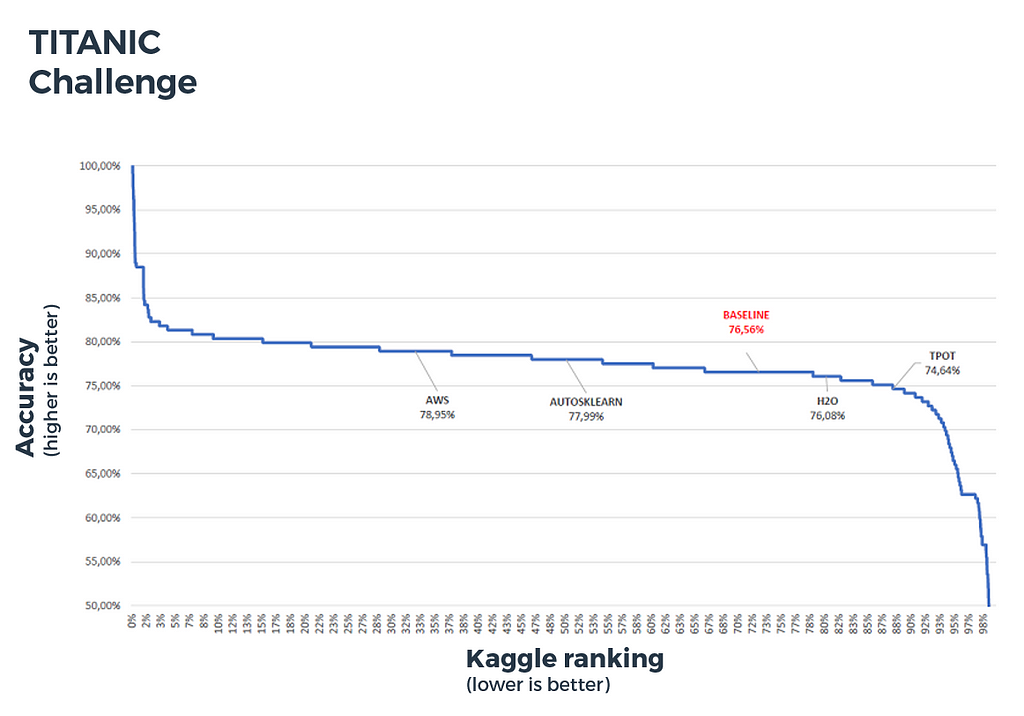Figure 5: Titanic challenge benchmark

This curve shows for instance that the top 20% solutions reached more than 80% accuracy.

MNIST (multiclass classification):

metric: accuracy
number of challengers: 2288 teams (2345 contributors)
number of features: 784
number of samples: 42000 in the training set, 28000 in the test set
baseline: k nearest neighbors with k=1

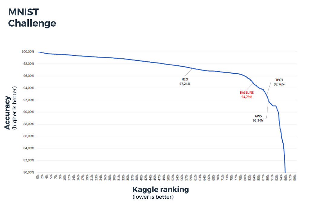Figure 6: MNIST challenge benchmark

House prices (regression):

metric: root mean squared error (RMSE)
number of challengers: 5123 teams (5397 competitors)
number of features: 268
number of samples: 1460 in the training set, 1459 in the test set
baseline: linear regression (area, number of bedrooms, year and month of sale)

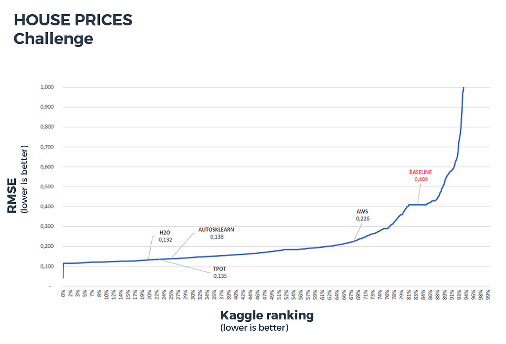Figure 7: House prices challenge benchmark

Conclusion

In practice, the open source frameworks needed some data preparation and cleaning (binarization, null values handling…). Only commercial solutions offer the complete pipeline, from features engineering to models deployment.

Moreover, hyperparameters tuning algorithms sometimes need to be parameterized. It is for instance the case for the genetic algorithm used by TPOT.

Open source Auto ML solutions does not perform better than human data scientists (top 20–80% on the leaderboard depending on the challenge) but can help get convenient levels of accuracy with a minimum effort and amount of time.

Keep in mind that feature engineering is the key:

“One of the holy grails of machine learning is to automate more and more of the feature engineering process” — Pedro Domingos, A Few Useful Things to Know about Machine Learning

This is where most of the effort in a machine learning project goes because it is a very time-consuming task.