Understanding YOLO

This article explains the YOLO object detection architecture, from the point of view of someone who wants to implement it from scratch. It will not describe the advantages/disadvantages of the network or the reasons for each design choice. Instead, it focus on how it works. You should have a basic understanding of neural networks, specially CNNS, before you read this.

All the descriptions in this post are related to the original YOLO paper: You Only Look Once: Unified, Real-Time Object Detection by Joseph Redmon, Santosh Divvala, Ross Girshick and Ali Farhadi (2015). There have been many improvements proposed since then, that were combined in the newer YOLOv2 version which I might write about another time. It is easier to understand this original version first, and then check what changes were made and why.

What is YOLO?

YOLO (You Only Look Once), is a network for object detection. The object detection task consists in determining the location on the image where certain objects are present, as well as classifying those objects. Previous methods for this, like R-CNN and its variations, used a pipeline to perform this task in multiple steps. This can be slow to run and also hard to optimize, because each individual component must be trained separately. YOLO, does it all with a single neural network. From the paper:

We reframe the object detection as a single regression problem, straight from image pixels to bounding box coordinates and class probabilities.

So, to put it simple, you take an image as input, pass it through a neural network that looks similar to a normal CNN, and you get a vector of bounding boxes and class predictions in the output.

So, what do these predictions look like?

The Predictions Vector

The first step to understanding YOLO is how it encodes its output. The input image is divided into an S x S grid of cells. For each object that is present on the image, one grid cell is said to be “responsible” for predicting it. That is the cell where the center of the object falls into.

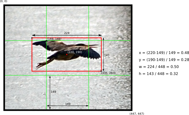
Each grid cell predicts B bounding boxes as well as C class probabilities. The bounding box prediction has 5 components: (x, y, w, h, confidence). The (x, y) coordinates represent the center of the box, relative to the grid cell location (remember that, if the center of the box does not fall inside the grid cell, than this cell is not responsible for it). These coordinates are normalized to fall between 0 and 1. The (w, h) box dimensions are also normalized to [0, 1], relative to the image size. Let’s look at an example:

Example of how to calculate box coordinates in a 448x448 image with S=3. Note how the (x,y) coordinates are calculated relative to the center grid cell

There is still one more component in the bounding box prediction, which is the confidence score. From the paper:

Formally we define confidence as Pr(Object) * IOU(pred, truth) . If no object exists in that cell, the confidence score should be zero. Otherwise we want the confidence score to equal the intersection over union (IOU) between the predicted box and the ground truth.

Note that the confidence reflects the presence or absence of an object of any class. In case you don't know what IOU is, take a look here.

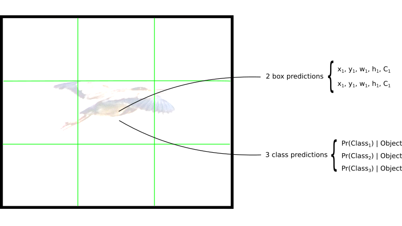
Now that we understand the 5 components of the box prediction, remember that each grid cell makes B of those predictions, so there are in total S x S x B * 5 outputs related to bounding box predictions.

It is also necessary to predict the class probabilities, Pr(Class(i) | Object). This probability is conditioned on the grid cell containing one object (see this if you don’t know that conditional probability means). In practice, it means that if no object is present on the grid cell, the loss function will not penalize it for a wrong class prediction, as we will see later. The network only predicts one set of class probabilities per cell, regardless of the number of boxes B. That makes S x S x C class probabilities in total

Adding the class predictions to the output vector, we get a S x S x (B * 5 +C) tensor as output.

Each grid cell makes B bounding box predictions and C class predictions (S=3, B=2 and C=3 in this example)

The Network

Once you understand how the predictions are encoded, the rest is easy. The network structure looks like a normal CNN, with convolutional and max pooling layers, followed by 2 fully connected layers in the end:

┌────────────┬────────────────────────┬───────────────────┐│    Name    │        Filters         │ Output Dimension  │├────────────┼────────────────────────┼───────────────────┤│ Conv 1     │ 7 x 7 x 64, stride=2   │ 224 x 224 x 64    ││ Max Pool 1 │ 2 x 2, stride=2        │ 112 x 112 x 64    ││ Conv 2     │ 3 x 3 x 192            │ 112 x 112 x 192   ││ Max Pool 2 │ 2 x 2, stride=2        │ 56 x 56 x 192     ││ Conv 3     │ 1 x 1 x 128            │ 56 x 56 x 128     ││ Conv 4     │ 3 x 3 x 256            │ 56 x 56 x 256     ││ Conv 5     │ 1 x 1 x 256            │ 56 x 56 x 256     ││ Conv 6     │ 1 x 1 x 512            │ 56 x 56 x 512     ││ Max Pool 3 │ 2 x 2, stride=2        │ 28 x 28 x 512     ││ Conv 7     │ 1 x 1 x 256            │ 28 x 28 x 256     ││ Conv 8     │ 3 x 3 x 512            │ 28 x 28 x 512     ││ Conv 9     │ 1 x 1 x 256            │ 28 x 28 x 256     ││ Conv 10    │ 3 x 3 x 512            │ 28 x 28 x 512     ││ Conv 11    │ 1 x 1 x 256            │ 28 x 28 x 256     ││ Conv 12    │ 3 x 3 x 512            │ 28 x 28 x 512     ││ Conv 13    │ 1 x 1 x 256            │ 28 x 28 x 256     ││ Conv 14    │ 3 x 3 x 512            │ 28 x 28 x 512     ││ Conv 15    │ 1 x 1 x 512            │ 28 x 28 x 512     ││ Conv 16    │ 3 x 3 x 1024           │ 28 x 28 x 1024    ││ Max Pool 4 │ 2 x 2, stride=2        │ 14 x 14 x 1024    ││ Conv 17    │ 1 x 1 x 512            │ 14 x 14 x 512     ││ Conv 18    │ 3 x 3 x 1024           │ 14 x 14 x 1024    ││ Conv 19    │ 1 x 1 x 512            │ 14 x 14 x 512     ││ Conv 20    │ 3 x 3 x 1024           │ 14 x 14 x 1024    ││ Conv 21    │ 3 x 3 x 1024           │ 14 x 14 x 1024    ││ Conv 22    │ 3 x 3 x 1024, stride=2 │ 7 x 7 x 1024      ││ Conv 23    │ 3 x 3 x 1024           │ 7 x 7 x 1024      ││ Conv 24    │ 3 x 3 x 1024           │ 7 x 7 x 1024      ││ FC 1       │ -                      │ 4096              ││ FC 2       │ -                      │ 7 x 7 x 30 (1470) │└────────────┴────────────────────────┴───────────────────┘

Some comments about the architecture:

• Note that the architecture was crafted for use in the Pascal VOC dataset, where the authors used S=7, B=2 and C=20. This explains why the final feature maps are 7x7, and also explains the size of the output (7x7x(2*5+20)). Use of this network with a different grid size or different number of classes might require tuning of the layer dimensions.
• The authors mention that there is a fast version of YOLO, with fewer convolutional layers. The table above, however, display the full version.
• The sequences of 1x1 reduction layers and 3x3 convolutional layers were inspired by the GoogLeNet (Inception) model
• The final layer uses a linear activation function. All other layers use a leaky RELU (Φ(x) = x, if x>0; 0.1x otherwise)
• If you are not familiar with convolutional networks, take a look at this great introduction

The Loss Function

There is a lot to say about the loss function, so let's do it by parts. It starts like this:

YOLO Loss Function — Part 1

This equation computes the loss related to the predicted bounding box position (x,y). Don’t worry about λ for now, just consider it a given constant. The function computes a sum over each bounding box predictor (j = 0.. B) of each grid cell (i = 0 .. S^2). 𝟙 obj is defined as follows:

• 1, If an object is present in grid cell i and the jth bounding box predictor is “responsible” for that prediction
• 0, otherwise

But how do we know which predictor is responsible for the object? Quoting the original paper:

YOLO predicts multiple bounding boxes per grid cell. At training time we only want one bounding box predictor to be responsible for each object. We assign one predictor to be “responsible” for predicting an object based on which prediction has the highest current IOU with the ground truth.

The other terms in the equation should be easy to understand: (x, y) are the predicted bounding box position and (x̂, ŷ) hat are the actual position from the training data.

Let’s move on to the second part:

YOLO Loss Function — Part 2

This is the loss related to the predicted box width / height. The equation looks similar to the first one, except for the square root. What’s up with that? Quoting the paper again:

Our error metric should reflect that small deviations in large boxes matter less than in small boxes. To partially address this we predict the square root of the bounding box width and height instead of the width and height directly.

Moving on to the third part:

YOLO Loss Function — Part 3

Here we compute the loss associated with the confidence score for each bounding box predictor. C is the confidence score and Ĉ is the intersection over union of the predicted bounding box with the ground truth.𝟙 obj is equal to one when there is an object in the cell, and 0 otherwise. 𝟙 noobj is the opposite.

The λ parameters that appear here and also in the first part are used to differently weight parts of the loss functions. This is necessary to increase model stability. The highest penalty is for coordinate predictions (λ coord = 5) and the lowest for confidence predictions when no object is present (λ noobj = 0.5).

The last part of the loss function is the classification loss:

YOLO Loss Function — Part 4

It looks similar to a normal sum-squared error for classification, except for the 𝟙 obj term. This term is used because so we don’t penalize classification error when no object is present on the cell (hence the conditional class probability discussed earlier).

The Training

The authors describe the training in the following way

• First, pretrain the first 20 convolutional layers using the ImageNet 1000-class competition dataset, using a input size of 224x224
• Then, increase the input resolution to 448x448
• Train the full network for about 135 epochs using a batch size of 64, momentum of 0.9 and decay of 0.0005
• Learning rate schedule: for the first epochs, the learning rate was slowly raised from 0.001 to 0.01. Train for about 75 epochs and then start decreasing it.
• Use data augmentation with random scaling and translations, and randomly adjusting exposure and saturation.

This procedure is described in deeper detail in the original paper. I plan to reproduce it myself, but I haven’t got there yet :).

Conclusion

It took me some time to get all the details about this paper. If you are reading this, I hope I made your job easier by sharing my comments about it.

I believe that the best test to check if you have really understood an algorithm is to try to implement it yourself from scratch. There are many details that are not explicit on the text and that you don’t realize until you get your hands dirty and try to build something with it.

Thanks for reading and please leve your comments below, if you have any.

Understanding YOLO was originally published in Hacker Noon on Medium, where people are continuing the conversation by highlighting and responding to this story.