8 Deep Learning Best Practices I Learned About in 2017

Something I was really happy about accomplishing in 2017 was getting more practically involved with modern AI. I’ve studied a lot of math, which has certainly been fun, but haven’t done any practical projects, and therefore have nothing to show for my efforts. To remedy this, in April, I applied for an AI Grant with the aim of building FastText skip-gram models for Kenyan speech. I became a finalist in the first round, but failed to win a grant.

Then, this September, I applied to the international fellowship track of a now-complete class on Practical Deep Learning for Coders, Part 1 v2, taught by Jeremy Howard of fast.ai. It will be publicly available as a MOOC in the first two weeks or so of January 2018. Over 7 weeks, I learned how to use a set of 8 techniques for building:

1. world-class image classifiers from pre-trained models,
2. sentiment analysis tools by building language models from the data sets under investigation,
3. how to do deep learning on structured data sets, and
4. how to use deep learning to build recommendation engines through collaborative filtering.

All this was done through the extremely productive interface known as the Jupyter Notebook, supported by the fastai deep learning library, which is itself supported by PyTorch.

So here are the 8 techniques. In each case, I’ll outline the general idea with short snippets of fastai code, and indicate (in parentheses) whether each technique is generally applicable (useful whether you’re doing DL for image recognition and classification, NLP, modeling structured data or collaborative filtering), or more specific to the kind of data you’re trying to apply deep learning to. During the class, the image recognition lessons were done using the Kaggle challenges Dogs vs. Cats: Kernels Edition, Dog Breed Identification, and Planet: Understanding the Amazon from Space.

Because this is the Internet, I made my own challenge, which was to clone Dogs vs. Cats, but with spiders and scorpions instead. Spiders vs. Scorpions. I grabbed the data from Google Images, by searching ‘spider’ and ‘desert scorpion’ and downloading about 1500 images or so. I automated this, obviously. I didn’t want to automatically become an expert on esoteric spiders and right-clicking. I cleaned up the data by removing any non-jpg images, any non-image cruft, and images that had no extension. By the time I was done filtering out the junk, I had about 815 images to work with. Each class [spiders, scorpions] had 290 in the training set, with 118 spiders and 117 scorpions in the test/validation set. Surprisingly (for me, when I learned this), it works! My model reached about 95% accuracy.

Transfer learning by fine-tuning VGG-16 and ResNext50. (computer vision and image classification)

For image classification work, you can get a lot of mileage by fine-tuning, for your specific problem, a neural network architecture that has done well on a more general challenge. An example is the residual network ResNext50, a 50-layer convolutional neural network. It was trained on the 1000 categories of the ImageNet challenge, and because it performed very well, the features it was able to extract from the image data are general enough to be reused. To get it to work for my problem domain, what I needed to do was replace the last layer, which outputs a 1000-dimensional vector of ImageNet predictions, with a layer which outputs a 2-dimensional vector. The two output classes are specified in the folder called PATH in the code snippet above. For the Spider vs. Scorpion challenge, I had the following:

$ ls -lsh data/spiderscorpions/train/128K drwxrwxrwx 1 bmn bmn 128K Jan  3 00:22 scorpions148K drwxrwxrwx 1 bmn bmn 148K Jan  3 00:22 spiders

Notice that the two contents of the train folder are themselves folders, each containing 290 images.

An example diagram of the fine-tuning procedure is shown here, which retrains a 10-dimensional final layer:

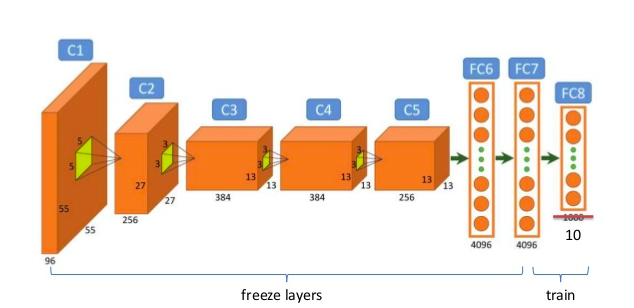Image obtained from hereCyclical Learning Rates (generally applicable)

The learning rate is probably the most important hyper-parameter to tune for training deep neural networks. The way it is typically done, in a non-adaptive setting (i.e. not using Adam, AdaDelta or their variants), is by a DL practitioner/researcher running, in parallel, multiple experiments, each with a small delta difference between learning rates. This takes a terribly long time if you have a large dataset and is quite error prone, if you are inexperienced in the ways of building intuition with stochastic matrices. However, in 2015, Leslie N. Smith, of the US Naval Research Laboratory, found a way to automatically search for the optimal learning rate by starting from a very small value, running a few mini-batches through the network, and tweaking the learning rate while tracking the change to the loss, until the loss starts decreasing. Two blog posts by fellow fast.ai students explaining the cyclical learning rates method are here and here.

In fastai, you take advantage of learning rate annealing by running lr_find() on your learner object, and sched.plot() to identify the point which coincides with the optimal learning rate. A screenshot:

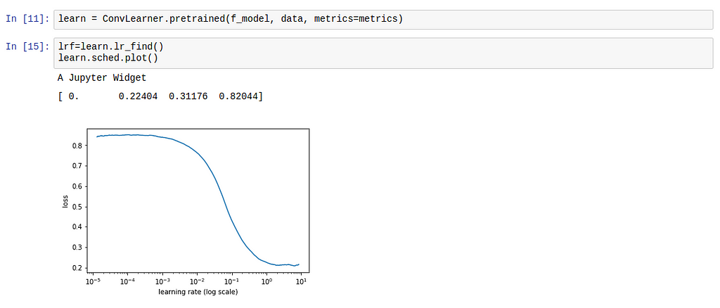0.1 seems like a good learning rate

An excerpt from the cyclical learning rate paper shows that it performs better, reaching the the highest accuracy, and more than twice as fast as letting the learning rate decay exponentially.

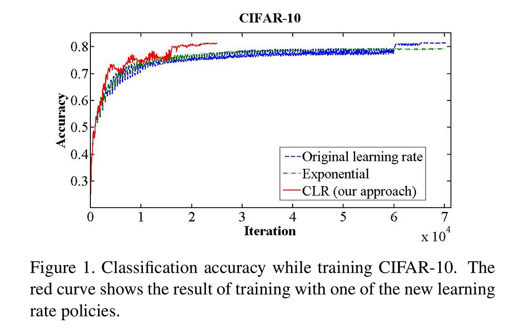Fig. 1: Smith (2017) “Cyclical learning rates for training neural networks.”Stochastic Gradient Descent with Restarts (generally applicable)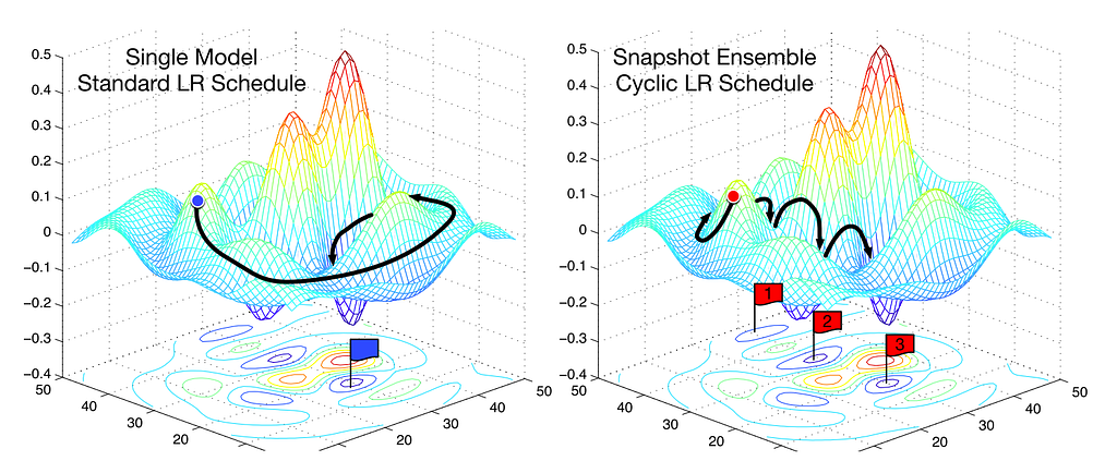Fig. 2: SGD vs. snapshot ensembles (Huang et al., 2017)

Another method for speeding up stochastic gradient descent involves gradually decreasing the learning rate as training progresses. What this helps with is noticing when changes to the learning rate coincide with improvements in the loss. As you get closer to the optimal weights, you want to take smaller steps, because if you take large steps you might skip the optimal region of the error surface. If the relationship between the learning rate and loss is unstable, i.e. if a small change to the learning rate results in a large change in the loss, then we’re not in a stable region (image 2 above). Then the strategy becomes to periodically increase the learning rate. The ‘period’ here is a number which determines how many times to increase the learning rate. This is the cyclical learning rate schedule. In fastai, this is set using cycle_len and cycle_mult params to learner.fit. In image 2 above, the learning rate is reset 3 times. It usually takes a much longer time to find the optimal loss when using the normal learning rate schedule, where a developer waits until all the epochs are complete before manually trying again with a different learning rate.

Data augmentation (computer vision and image classification — for now)

Data augmentation is a simple method for increasing the amount of training and test data you have. For images, this depends on the learning problem at hand, and therefore on the number of symmetries in the images in the dataset. An example is the Spiders vs. Scorpions toy challenge. Many pictures in this dataset could be reflected vertically and still show the animal without weird distortions. This is called transforms_side_on. Example:

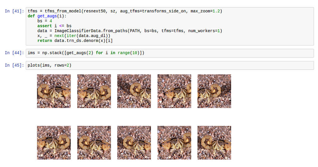From top to bottom, notice the different angles, zoom and reflections.Test-time augmentation (computer vision and image classification — for now)

We can also use data augmentation at inference time (or test time, hence the name). At inference time, all you’re doing is making predictions. You could do it with the individual images in the test set, but the process becomes more robust if randomly generate a few augmentations of each image in the test set that is accessed. In fastai, 4 random augmentations per test image are used in the predictions, and the average of those predictions is used as the prediction for that image.

Replace word vectors with a pretrained recurrent neural network

A way to get a world-class sentiment analysis framework, without using word vectors, is to take the entire training data set that you intend to analyze and build a deep recurrent neural network language model from it. Save the model’s encoder when the model has high accuracy and use the embeddings you get from the encoder to build a sentiment analysis model. This works better than the embedding matrices one gets from word vectors because RNNs can keep track of long range dependencies better than word vectors.

Back-propagation through time (BPTT) (NLP)

The hidden state in a deep recurrent neural network can grow to an unwieldy size if it isn’t reset after back-propagating some time-steps. For example, in a character-level RNN, if you have a million characters, then you also have a million hidden state vectors, each with their history. To adjust the gradients of the neural network, we then need to perform 1 million computations of the chain rule per character, per batch. This will consume too much memory. So, to lower the memory requirements, we set a maximum number of characters to back-propagate to. Since each loop in a recurrent neural network is known as a time-step, the task of limiting the number of layers through which back-propagation retains the history of the hidden state is called back-propagation through time. The value of this number determines the time and memory requirements of the model’s computation, but it improves the model’s ability to handle long sentences or sequences of actions.

Entity embedding of categorical variables. (Structured Data and NLP)

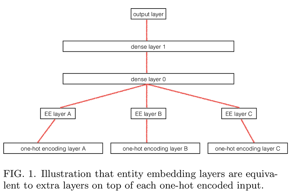
When doing deep learning on structured data-sets, it helps to distinguish columns that contain continuous data, such as price information in an online store, from columns that contain categorical data, e.g. dates and pick-up locations. One can then convert the one-hot encoding process for these categorical columns into a look-up table that points to an fully-connected embedding layer of a neural network. Your neural network therefore gets an opportunity to learn things about those categorical variables/columns that would have been ignored had the categorical nature of the columns been ignored. It can learn cyclical events, such as which days of the week have the most sales, what happens just before public holidays and just after, for multi-year data-sets. The end-result of this is a very effective method for predicting optimal pricing for products and collaborative filtering. This should be a standard data analysis and prediction method for all companies that have tabular data. Which is all of them. All companies should be using this.

This method was applied in the Rossmann Store Sales Kaggle competition by Guo and Berkhahn, which got them to third place even if they only used deep learning with minimal feature engineering. They outlined their method in this paper.

Guo, Berkhahn (2016)Fin.

The deep learning sub-field of AI is getting easier and easier to get into, as libraries get better. It feels like researchers and practitioners have hill-climbed their way, with bigger and bigger strides, enabled by hard work compiling large data sets and capable GPUs, to the grand achievement of releasing, in the open, a set of tools that promise to upend the course of human history. To my mind, the greatest potential lies in education and medicine, especially rejuvenation biotechnology. Even before we use deep learning to create artificial general intelligence, with the right policy, insight, motivation and global coordination, we’ll be smarter, richer, and should expect to live much, much longer, healthier lives by the end of this century because of these tools.

8 Deep Learning Best Practices I Learned About in 2017 was originally published in Hacker Noon on Medium, where people are continuing the conversation by highlighting and responding to this story.