One Class Classification for Images with Deep features

As programmers we regularly come across projects that require the task of building binary classifiers of the types A vs ~A, in which when the classifier is given a new data sample, it’s able to predict whether the sample belongs to class A or is an outlier. One reliable but difficult approach to solve such a problem is using the One-class Learning Paradigm.

In one-class learning we train the model only on the positive class data-set and take judgments from it on the universe [A union ~A] spontaneously. It’s a hot research topic and there are multiple tools available, like One-class SVM and Isolation Forest, to achieve this task. One-class learning can prove to be vital in scenarios where data consisting of ~A samples can take up any distribution and it isn’t possible to learn a pattern for ~A class.

But one-class learning becomes more challenging when the dimensions of the sample points increase. For example, consider an image size of 224x224px — to apply any one-class learning algorithm here straight out of the box can prove fatal due to the immense number of features each sample point holds (in this example it’s 50,176 features). Consequently efficient and discriminating feature representation is required to build a one-class classifier for images or high-dimensional data in general.

This post covers the implementation of one-class learning using deep neural net features and compares classifier performance based on the approaches of OC- SVM, Isolation Forest and Gaussian Mixtures.

CNNs as Feature Extractors

Convolutional Neural Nets have proven to be state-of-the-art when it comes to object recognition in images. CNNs have replaced traditional machine learning pipelines where feature extraction and the models used to learn from those features were two separate entities. Moreover, CNNs can also help in extraction of meaningful features for an image because a deep neural net also learns which features are important and which aren’t, in order to distinguish a class from the others. This allows us to simply use features returned from these deep CNNs which are ready-to-go, and build our classifier.

Moreover, the availability of pre-trained CNNs on ImageNet data, with over 1,000 categories and more than 14 million images, has made image categorization much more simple since a pre-trained CNN will generally return features which are sufficiently satisfactory to train a light-weight model using them.

As I mentioned earlier — since feature vectors returned by CNNs give powerful representation of the image which generated them, we use these features to train our one-class classifier. For the purpose of this post, we use ResNet-50 as feature extractor for our model. Why? Because it’s fast, accurate, and credible as it won the ImageNet Challenge in 2015.

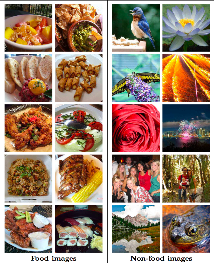
Dataset used for this problem — We use the Food5k data-set, which contains both Food and ~Food images (2500 each). Sample images are shown below -

Sample food vs ~food images

Implementation details for One Class SVM and Isolation Forest models:

We first compute ResNet-50 features for the image data-set. The code for which will look as follows -

from keras.applications.resnet50 import ResNet50def extract_resnet(X):      # X : images numpy array    resnet_model = ResNet50(input_shape=(image_h, image_w, 3), weights='imagenet', include_top=False)  # Since top layer is the fc layer used for predictions    features_array = resnet_model.predict(X)    return features_array

We can accordingly compute ResNet features for all the images in the data-set. Next step, follow the pipeline -

1. Apply standard scaler on the obtained features.
2. Principal Component Analysis with n_components = 512.
3. Pass the remaining features to One Class SVM model or Isolation Forest

In below code, X_train and X_test are the resnet features for the train and test images.

from sklearn.preprocessing import StandardScalerfrom sklearn.decomposition import PCAfrom sklearn.ensemble import IsolationForestfrom sklearn import svm# Apply standard scaler to output from resnet50ss = StandardScaler()ss.fit(X_train)X_train = ss.transform(X_train)X_test = ss.transform(X_test)# Take PCA to reduce feature space dimensionalitypca = PCA(n_components=512, whiten=True)pca = pca.fit(X_train)print('Explained variance percentage = %0.2f' % sum(pca.explained_variance_ratio_))X_train = pca.transform(X_train)X_test = pca.transform(X_test)# Train classifier and obtain predictions for OC-SVMoc_svm_clf = svm.OneClassSVM(gamma=0.001, kernel='rbf', nu=0.08)  # Obtained using grid searchif_clf = IsolationForest(contamination=0.08, max_features=1.0, max_samples=1.0, n_estimators=40)  # Obtained using grid searchoc_svm_clf.fit(X_train)if_clf.fit(X_train)oc_svm_preds = oc_svm_clf.predict(X_test)if_preds = if_clf.predict(X_test)# Further compute accuracy, precision and recall for the two predictions sets obtained

PS: Predictions returned by both isolation forest and one-class SVM are of the form {-1, 1}. -1 for the “Not food” and 1 for “Food”.

One Class Classification using Gaussian Mixtures and Isotonic Regression

Intuitively, food items can belong to different clusters like cereals, egg dishes, breads, etc., and some food items may also belong to multiple clusters simultaneously. As a result, we can fit a Gaussian mixture on the positive class data points (ResNet features). Gaussian mixture models “are a probabilistic model for representing normally distributed subpopulations within an overall population”. It can be surmised that a mixture model represents clusters of normally distributed subpopulations. A Gaussian mixture model, once fitted on the data, can give us information on the probability of whether any new point was generated from that distribution.

But beware — Gaussian mixture models return log of probability density function values for a given sample (and not actual probabilities). Hence it is necessary to convert these probability density function values to ‘probability scores’, which can then show that a new sample will belong to the Gaussian distribution with “x” amount of confidence.

A simple yet efficient method to accomplish this is by fitting an isotonic regression model on the log probability density scores w.r.t. labels for the validation set data points. Isotonic regression is a probability calibration technique which can calibrate classifier scores to approximate probability values by fitting a stepwise non-decreasing function along the scores returned by the classifier.

Implementation Details for one class learning with GMMs

# The standard scaler and PCA part remain same. Just that we will also require a validation set to fit# isotonic regressor on the probability density scores returned by GMM# Also assuming that resnet feature generation is donefrom sklearn.mixture import GaussianMixturefrom sklearn.isotonic import IsotonicRegression

gmm_clf = GaussianMixture(covariance_type='spherical', n_components=18, max_iter=int(1e7))  # Obtained via grid search

gmm_clf.fit(X_train)

log_probs_val = gmm_clf.score_samples(X_val)

isotonic_regressor = IsotonicRegression(out_of_bounds='clip')isotonic_regressor.fit(log_probs_val, y_val)  # y_val is for labels 0 - not food 1 - food (validation set)# Obtaining results on the test setlog_probs_test = gmm_clf.score_samples(X_test)test_probabilities = isotonic_regressor.predict(log_probs_test)test_predictions = [1 if prob >= 0.5 else 0 for prob in test_probabilities]# Calculate accuracy metrics

Results and Discussions

Following are the results obtained using the three one class learning techniques

Results table comparing all three algorithms over food vs ~food data

Thus the GMM model (calibrated using isotonic regression) outperforms both the other one-class learning models and is not far from ‘state-of-art’ which is obtained after training a neural net for 700 iterations. Furthermore, in the state-of-art approach the model is trained on both positive and negative data samples, whereas in our approach the model is just trained on positive class samples, therefore making it more robust to handle any kind of distributions in the ~A samples.

GMM helps improve the precision of the model by correctly predicting more “Not food” images as compared to one-class SVM. This results in considerable less false positives. For example, some of the images for which GMM correctly predicts as “Not food” (as opposed to OC-SVM) are -

Not food correctly predicted by GMM as opposed to OC-SVM

Finishing off with an additional note — I didn’t go deeper on how to do a grid search for Gaussian Mixture Models but anyone who wishes to read in more about it can check out this sklearn tutorial.

If you liked this post you can check more stories from Squad Engineering at https://medium.com/squad-engineering.

One Class Classification for Images with Deep features was originally published in Hacker Noon on Medium, where people are continuing the conversation by highlighting and responding to this story.